SQL.ppt

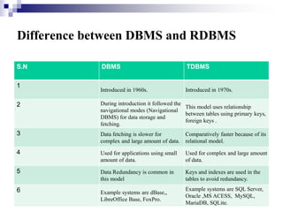
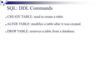
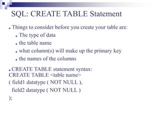
SQL(Structured Query
Language)

Overview
Introduction
DDL Commands
DML Commands
SQL Statements, Operators, Clauses
Aggregate Functions

Difference between DBMS and RDBMS
S.N DBMS TDBMS
1
Introduced in 1960s. Introduced in 1970s.
2 During introduction it followed the
navigational modes (Navigational
DBMS) for data storage and
fetching.
This model uses relationship
between tables using primary keys,
foreign keys .
3 Data fetching is slower for
complex and large amount of data.
Comparatively faster because of its
relational model.
4 Used for applications using small
amount of data.
Used for complex and large amount
of data.
5 Data Redundancy is common in
this model
Keys and indexes are used in the
tables to avoid redundancy.
6 Example systems are dBase,,
LibreOffice Base, FoxPro.
Example systems are SQL Server,
Oracle ,MS ACESS, MySQL,
MariaDB, SQLite.

The ANSI standard language for the definition and
manipulation of relational database.
Includes data definition language (DDL), statements that
specify and modify database schemas.
Includes a data manipulation language (DML), statements
that manipulate database content.
Structured Query Language (SQL)

Some Facts on SQL
SQL data is case-sensitive, SQL commands are not.
First Version was developed at IBM by Donald D.
Chamberlin and Raymond F. Boyce. [SQL]
Developed using Dr. E.F. Codd's paper, “A Relational Model
of Data for Large Shared Data Banks.”
SQL query includes references to tuples variables and the
attributes of those variables

SQL: DDL Commands
CREATE TABLE: used to create a table.
ALTER TABLE: modifies a table after it was created.
DROP TABLE: removes a table from a database.

SQL: CREATE TABLE Statement
Things to consider before you create your table are:
The type of data
the table name
what column(s) will make up the primary key
the names of the columns
CREATE TABLE statement syntax:
CREATE TABLE <table name>
( field1 datatype ( NOT NULL ),
field2 datatype ( NOT NULL )
);

SQL: ALTER TABLE Statement
To add or drop columns on existing tables.
ALTER TABLE statement syntax:
ALTER TABLE <table name>
ADD attr datatype;
or
DROP COLUMN attr;

SQL: DROP TABLE Statement
DROP TABLE statement syntax:
DROP TABLE <table name> ;

Example:
CREATE TABLE FoodCart (
date varchar(10),
food varchar(20),
profit float
);
ALTER TABLE FoodCart (
ADD sold int
);
ALTER TABLE FoodCart(
DROP COLUMN profit
);
DROP TABLE FoodCart;
profit
food
date
sold
profit
food
date
sold
food
date
FoodCart
FoodCart
FoodCart

SQL: DML Commands
INSERT: adds new rows to a table.
UPDATE: modifies one or more attributes.
DELETE: deletes one or more rows from a table.

SQL: INSERT Statement
To insert a row into a table, it is necessary to have a value
for each attribute, and order matters.
INSERT statement syntax:
INSERT into <table name>
VALUES ('value1', 'value2', NULL);
Example: INSERT into FoodCart
VALUES (’02/26/08', ‘pizza', 70 );
FoodCart
70
pizza
02/26/08
500
hotdog
02/26/08
350
pizza
02/25/08
sold
food
date
500
hotdog
02/26/08
350
pizza
02/25/08
sold
food
date

SQL: UPDATE Statement
To update the content of the table:
UPDATE statement syntax:
UPDATE <table name> SET <attr> = <value>
WHERE <selection condition>;
Example: UPDATE FoodCart SET sold = 349
WHERE date = ’02/25/08’AND food = ‘pizza’;
FoodCart
70
pizza
02/26/08
500
hotdog
02/26/08
350
pizza
02/25/08
sold
food
date
70
pizza
02/26/08
500
hotdog
02/26/08
349
pizza
02/25/08
sold
food
date

SQL: DELETE Statement
To delete rows from the table:
DELETE statement syntax:
DELETE FROM <table name>
WHERE <condition>;
Example: DELETE FROM FoodCart
WHERE food = ‘hotdog’;
FoodCart
Note: If the WHERE clause is omitted all rows of data are deleted from the table.
70
pizza
02/26/08
500
hotdog
02/26/08
349
pizza
02/25/08
sold
food
date
70
pizza
02/26/08
349
pizza
02/25/08
sold
food
date

SQL Statements, Operations, Clauses
SQL Statements:
Select
SQL Operations:
Join
Left Join
Right Join
Like
SQL Clauses:
Order By
Group By
Having

SQL: SELECT Statement
A basic SELECT statement includes 3 clauses
SELECT <attribute name> FROM <tables> WHERE <condition>
SELECT
Specifies the attributes
that are part of the
resulting relation
FROM
Specifies the tables
that serve as the input
to the statement
WHERE
Specifies the selection
condition, including
the join condition.

Using a “*” in a select statement indicates that every
attribute of the input table is to be selected.
Example: SELECT * FROM … WHERE …;
To get unique rows, type the keyword DISTINCT after
SELECT.
Example: SELECT DISTINCT * FROM …
WHERE …;
SQL: SELECT Statement (cont.)

Example:
Person
80
34
Peter
54
54
Helena
70
29
George
64
28
Sally
80
34
Harry
Weight
Age
Name
80
34
Peter
54
54
Helena
80
34
Harry
Weight
Age
Name
80
54
80
Weight
1) SELECT *
FROM person
WHERE age > 30;
2) SELECT weight
FROM person
WHERE age > 30;
3) SELECT distinct weight
FROM person
WHERE age > 30;
54
80
Weight

SQL: Join operation
A join can be specified in the FROM clause which
list the two input relations and the WHERE clause
which lists the join condition.
Example:
Biotech
1003
Sales
1002
IT
1001
Division
ID
TN
1002
MA
1001
CA
1000
State
ID
Emp Dept

SQL: Join operation (cont.)
Sales
1002
IT
1001
Dept.Division
Dept.ID
TN
1002
MA
1001
Emp.State
Emp.ID
inner join = join
SELECT *
FROM emp join dept (or FROM emp, dept)
on emp.id = dept.id;

IT
1001
Sales
1002
null
null
Dept.Division
Dept.ID
CA
1000
TN
1002
MA
1001
Emp.State
Emp.ID
left outer join = left join
SELECT *
FROM emp left join dept

Sales
1002
Biotech
1003
IT
1001
Dept.Division
Dept.ID
MA
1001
null
null
TN
1002
Emp.State
Emp.ID
right outer join = right join
SELECT *
FROM emp right join dept

SQL: Like operation
Pattern matching selection
% (arbitrary string)
SELECT *
FROM emp
WHERE ID like ‘%01’;
finds ID that ends with 01, e.g. 1001, 2001, etc
_ (a single character)
SELECT *
FROM emp
WHERE ID like ‘_01_’;
finds ID that has the second and third character as 01, e.g.
1010, 1011, 1012, 1013, etc

SQL: The ORDER BY Clause
Ordered result selection
desc (descending order)
SELECT *
FROM emp
order by state desc
puts state in descending order, e.g. TN, MA, CA
asc (ascending order)
SELECT *
FROM emp
order by id asc
puts ID in ascending order, e.g. 1001, 1002, 1003

SQL: The GROUP BY Clause
The function to divide the tuples into groups and returns an
aggregate for each group.
Usually, it is an aggregate function’s companion
SELECT food, sum(sold) as totalSold
FROM FoodCart
group by food;
FoodCart
419
pizza
500
hotdog
totalSold
food
70
pizza
02/26/08
500
hotdog
02/26/08
349
pizza
02/25/08
sold
food
date

SQL: The HAVING Clause
The substitute of WHERE for aggregate functions
Usually, it is an aggregate function’s companion
SELECT food, sum(sold) as totalSold
FROM FoodCart
group by food
having sum(sold) > 450;
FoodCart
500
hotdog
totalSold
food
70
pizza
02/26/08
500
hotdog
02/26/08
349
pizza
02/25/08
sold
food
date

SQL: Aggregate Functions
Are used to provide summarization information for SQL
statements, which return a single value.
COUNT(attr)
SUM(attr)
MAX(attr)
MIN(attr)
AVG(attr)
Note: when using aggregate functions, NULL values are not
considered, except in COUNT(*) .

SQL: Aggregate Functions (cont.)
COUNT(attr) -> return # of rows that are not null
Ex: COUNT(distinct food) from FoodCart; -> 2
SUM(attr) -> return the sum of values in the attr
Ex: SUM(sold) from FoodCart; -> 919
MAX(attr) -> return the highest value from the attr
Ex: MAX(sold) from FoodCart; -> 500
70
pizza
02/26/08
500
hotdog
02/26/08
349
pizza
02/25/08
sold
food
date
FoodCart

SQL: Aggregate Functions (cont.)
MIN(attr) -> return the lowest value from the attr
Ex: MIN(sold) from FoodCart; -> 70
AVG(attr) -> return the average value from the attr
Ex: AVG(sold) from FoodCart; -> 306.33
Note: value is rounded to the precision of the datatype
70
pizza
02/26/08
500
hotdog
02/26/08
349
pizza
02/25/08
sold
food
date
FoodCart

SQL.ppt

SQL.ppt

More Related Content

What's hot

Similar to SQL.ppt

More from Ranjit273515

Recently uploaded

SQL.ppt