Linear Programming Simplex method -I
Introduction:
The geometric method of solving linear programming problems
presented before.
The graphical method is useful only for problems involving two decision
variables and relatively few problem constraints.
Simplex method is the most popular method used for the solution of
Linear Programming Problems (LPP).
What happens when we need more decision variables and more problem constraints?
We use an algebraic method called the simplex method, which was
developed by George B. DANTZIG (1914-2005) in 1947 while on
assignment with the U.S. Department of the air force.
Linear Programming Simplex method -I
 Motivation of Simplex method
 Solution of a LPP, if exists, lies at one of the vertices of the feasible region.
 All the basic solutions can be investigated one-by-one to pick up the optimal
solution.
 For 10 equations with 15 variables there
exists
basic feasible solutions!
Too large number to investigate one-by-one.
This can be overcome by simplex method
3003
10
15

C
General procedure of simplex method
 Simplex method involves following steps
1.General form of given LPP is transformed to its
canonical form.
2.Find a basic feasible solution of the LPP .
3.Move to an adjacent basic feasible solution which is closest to the optimal
solution among all other adjacent vertices.
4.Repeat until optimum solution is achieved.
Step three involves ‘ Simplex Algorithm’
4
Standard Form of a Linear
Programming Problem
Scalar form
ariables
decision v
the
are
and
constants,
known
are
)
,
,
2
,
1
;
,
,
2
,
1
(
and
,
where
0
0
0
s
constraint
the
subject to
)
,
,
,
(
Minimize
2
1
2
2
1
1
2
2
2
22
1
21
1
1
2
12
1
11
2
2
1
1
2
1
j
ij
j
j
n
m
n
mn
m
m
n
n
n
n
n
n
n
x
n
j
m
i
a
b
c
x
x
x
b
x
a
x
a
x
a
b
x
a
x
a
x
a
b
x
a
x
a
x
a
x
c
x
c
x
c
x
x
x
f






























5
Standard Form of a Linear
Programming Problem
Matrix form





























































mn
m
m
m
n
n
n
m
n
a
a
a
a
a
a
a
a
a
a
a
a
c
c
c
b
b
b
x
x
x
f







3
2
1
2
23
22
21
1
13
12
11
2
1
2
1
2
1
,
,
where
0
s
constraint
the
subject to
)
(
Minimize
a
c
b
X
X
b
aX
X
cT
X
6
Characteristic of a Linear
Programming Problem
• The objective function is of the minimization type
• All the constraints are of the equality type
• All the decision variables are nonnegative
• The number of the variables in the problem is n. This includes
the slack and surplus variables.
• The number of constraints is m (m < n).
7
Characteristic of a Linear
Programming Problem
• The number of basic variables is m (same as the number of constraints).
• The number of nonbasic variables is n-m.
• The column of the right hand side b is positive and greater than or equal to
zero.
• The calculations are organized in a table.
• Only the values of the coefficients are necessary for the calculations. The
table therefore contains only coefficient values, the matrix A in previous
discussions. These are the coefficients in the constraint equations.
• The objective function is the last row in the table. The constraint
coefficients are written first.
• Row operations consist of adding (subtracting)a definite multiple of the
pivot row from other rows of the table.
8
Transformation of LP Problems into
Standard Form
• The maximization of a function f(x1,x2,…,xn ) is equivalent to the minimization
of the negative of the same function. For example, the objective function
• Consequently, the objective function can be stated in the minimization form in
any linear programming problem.
n
n
n
n
x
c
x
c
x
c
f
f
x
c
x
c
x
c
f














2
2
1
1
2
2
1
1
maximize
to
equivalent
is
minimize
9
Transformation of LP Problems into
Standard Form
• A variable may be unrestricted in sign in some problems. In such cases, an
unrestricted variable (which can take a positive, negative or zero value) can be
written as the difference of two nonnegative variables.
• Thus if xj is unrestricted in sign, it can be written as xj=xj'-xj", where
• It can be seen that xj will be negative, zero or positive, depending on whether xj" is
greater than, equal to, or less than xj
’
.
0
"
and
0
' 
 j
j x
x
10
Transformation of LP Problems into
Standard Form
If a constraint appears in the form of a “less than or equal to” type of inequality as:
It can be converted into the equality form by adding a nonnegative slack variable xn+1 as
follows:
k
n
kn
k
k b
x
a
x
a
x
a 


 
2
2
1
1
k
n
n
kn
k
k b
x
x
a
x
a
x
a 



 1
2
2
1
1 
11
Transformation of LP Problems into
Standard Form
If a constraint appears in the form of a “greater than or equal to” type of inequality
as:
it can be converted into the equality form by subtracting a variable as:
where xn+1 is a nonnegative variable known as a surplus variable.
k
n
kn
k
k b
x
a
x
a
x
a 


 
2
2
1
1
k
n
n
kn
k
k b
x
x
a
x
a
x
a 



 1
2
2
1
1 
SIMPLEX METHOD
Step-1
Write the
standard
maximization
problem in
canonical form,
introduce slack
variables to
form the initial
system, and
write the initial
tableau.
Step-3
Select
the
pivot
column
Step-5
Select
the
pivot
element
and
perform
the
pivot
operatio
n
STOP
The optimal solution has been
found.
STOP
The linear programming problem
has no optimal solution
Step 2
Are there
any
negative
indicators
in the
bottom/t
oprow?
Step 4
Are there
any
positive
elements
in the
pivot
column
above the
dashed
line?
Simplex algorithm for standard maximization problems
NO
Yes
To solve a linear programming problem in standard form, use the
following steps.
1- Convert each inequality in the set of constraints to an equation by adding
slack variables.
2- Create the initial simplex tableau.
3- Select the pivot column. ( The column with the “most negative value”
element in the first/last row.)
4- Select the pivot row. (The row with the smallest non-negative result
when the last element in the row is divided by the corresponding in the
pivot column.)
5-Use elementary row operations calculate new values for the pivot row so
that the pivot is 1 (Divide every number in the row by the pivot number.)
6- Use elementary row operations to make all numbers in the pivot column
equal to 0 except for the pivot number.
If all entries in the first/bottom row are zero or positive, this the final
tableau. If not, go back to step 3.
7- If you obtain a final tableau, then the linear programming problem has a
maximum solution, which is given by the entry in the lower-right corner
of the tableau.
Simplex Algorithm
 Let us consider the following LPP
0
,
,
4
2
2
5
0
2
4
6
2
2
2
4
3
2
1
3
2
1
3
2
1
3
2
1
3
2
1













x
x
x
x
x
x
x
x
x
x
x
x
to
Subject
x
x
x
Z
Maximize
Simplex Algorithm…contd.
 LPP is transformed to its standard form
 Note that x4, x5, x6 are slack variables.
0
,
,
,
,
,
4
2
2
5
0
2
4
6
2
2
2
4
6
5
4
3
2
1
6
3
2
1
5
3
2
1
4
3
2
1
3
2
1
















x
x
x
x
x
x
x
x
x
x
x
x
x
x
x
x
x
x
to
Subject
x
x
x
Z
Maximize
Simplex Algorithm …contd.
Set of equations, including the objective function is transformed to
canonical form
Basic feasible solution of above canonical form is
x4 = 6, x5= 0, x6= 4, x1= x2= x3= 0 and Z = 0
x4, x5, x6 : Basic Variables ; x1, x2, x3 : Non-basic Variables
4
1
0
0
2
2
5
0
0
1
0
2
4
6
0
0
1
2
2
0
0
0
0
2
4
6
5
4
3
2
1
6
5
4
3
2
1
6
5
4
3
2
1
6
5
4
3
2
1


























x
x
x
x
x
x
x
x
x
x
x
x
x
x
x
x
x
x
Z
x
x
x
x
x
x
Simplex Algorithm …contd.
 Symbolized form
 The left-most column is known as basis as this is consisting of basic
variables
 The coefficients in the first row (c1,…..c6) are known as cost coefficients.
 
 
 
  6
6
66
5
65
4
64
3
63
2
62
1
61
6
5
6
56
5
55
4
54
3
53
2
52
1
51
5
4
6
46
5
45
4
44
3
43
2
42
1
41
4
6
6
5
5
4
4
3
3
2
2
1
1
b
x
c
x
c
x
c
x
c
x
c
x
c
x
b
x
c
x
c
x
c
x
c
x
c
x
c
x
b
x
c
x
c
x
c
x
c
x
c
x
c
x
b
Z
x
c
x
c
x
c
x
c
x
c
x
c
Z

























Simplex Algorithm …contd.
 This completes first step of algorithm.
 After completing each step (iteration) of algorithm, following three
points are to be examined:
1.Is there any possibility of further improvement?
2.Which non basic variable is to be entered into the basis?
3.Which basic variable is to be exited from the basis?
Simplex Algorithm …contd.
 Is there any possibility of further improvement?
If any one of the cost coefficients is negative further improvement is
possible.
 Which non basic variable is to be entered?
Entering variable is decided such that the unit change of this variable
should have maximum effect on the objective function. Thus the variable
having the coefficient which is minimum among all cost coefficients is to
be entered, i.e., xs is to be entered if cost coefficient cs is minimum.
Simplex Algorithm …contd.
 Which basic variable is to be exited ?
After deciding the entering variable xs , xr (from the set of basic variables)
is decided to be the exiting variable if
is minimum for all possible r, provided crs is positive. crs
is considered as pivotal element to obtain the next canonical form.
s
r
r
c
b
Simplex Algorithm …contd.
 Entering variable
c1is minimum (-4), thus, x1is the entering variable for the next step of
calculation.
 Exiting variable
r may take any value from 4, 5 and 6. It is found that ,
As,
is minimum, r is 5. Thus, x5 is to be exited.c51 ( = 1) is considered as
pivotal element and x5 is replaced by x1 in the basis.
Thus a new canonical form is obtained through pivotal operation.
8
.
0
5
4
,
0
1
0
,
3
2
6
61
6
51
5
41
4






c
b
c
b
c
b
51
5
c
b
Simplex Algorithm …contd.
 After the pivotal operation, the canonical form
obtained as follows
The Basic feasible solution of above canonical form is
x1 = 0, x4 = 6, x6= 4, x2= x3= x5 = 0 and Z = 0
Note that cost coefficient c2 is negative. Thus optimum
solution is not yet achieved. Further improvement is
possible.
 
 
 
  4
1
5
0
12
18
0
0
0
1
0
2
4
1
6
0
2
1
2
9
0
0
0
4
0
6
15
0
6
5
4
3
2
1
6
6
5
4
3
2
1
1
6
5
4
3
2
1
4
6
5
4
3
2
1

























x
x
x
x
x
x
x
x
x
x
x
x
x
x
x
x
x
x
x
x
x
Z
x
x
x
x
x
x
Z
Simplex Algorithm …contd.
 Entering variable
c2is minimum (-15), thus, x2 is the entering variable for the next step of
calculation.
 Exiting variable
r may take any value from 4, 1 and 6. However, c12is negative (-4). Thus, r
may be either 4 or 6. It is found that,
As,
is minimum, r is 6. Thus, x6 is to be exited.c62 ( = 18) is considered as
pivotal element and x6 is replaced by x2 in the basis.
Thus another canonical form is obtained.
222
.
0
18
4
,
667
.
0
9
6
62
6
42
4




c
b
c
b
62
6
c
b
Simplex Algorithm …contd.
 After the pivotal operation, the canonical form
obtained as follows
 
 
 
 
9
2
18
1
18
5
0
3
2
1
0
9
8
9
2
9
1
0
3
2
0
1
4
2
1
2
1
1
4
0
0
3
10
6
5
6
1
0
4
0
0
6
5
4
3
2
1
2
6
5
4
3
2
1
1
6
5
4
3
2
1
4
6
5
4
3
2
1

























x
x
x
x
x
x
x
x
x
x
x
x
x
x
x
x
x
x
x
x
x
Z
x
x
x
x
x
x
Z
Simplex Algorithm …contd.
The Basic feasible solution of above
canonical form is
Note that cost coefficient c3 is negative.
Thus optimum solution is not yet
achieved. Further improvement is
possible.
3
10
,
0
,
0
,
0
,
4
,
9
2
,
9
8
6
5
3
4
2
1 





 Z
and
x
x
x
x
x
x
Simplex Algorithm …contd.
 Entering variable
x3 is the entering variable for the next step of calculation.
 Exiting variable
x4 is the exiting variable.c43 ( = 4) is considered as pivotal element and x4
is replaced by x3 in the basis.
Thus another canonical form is obtained.
Simplex Algorithm …contd.
 After the pivotal operation, the canonical form
obtained as follows
 
 
 
 
9
8
36
1
36
7
6
1
0
1
0
9
14
36
5
36
1
6
1
0
0
1
1
8
1
8
1
4
1
1
0
0
3
22
3
1
3
1
1
0
0
0
6
5
4
3
2
1
2
6
5
4
3
2
1
1
6
5
4
3
2
1
3
6
5
4
3
2
1

























x
x
x
x
x
x
x
x
x
x
x
x
x
x
x
x
x
x
x
x
x
Z
x
x
x
x
x
x
Z
Simplex Algorithm …contd.
 The basic solution of above canonical form is
 Note that all the cost coefficients are nonnegative. Thus the optimum
solution is achieved.
 Optimum solution is
3
22
,
0
,
0
,
0
,
1
,
9
8
,
9
14
6
5
4
3
2
1 





 Z
and
x
x
x
x
x
x
1
,
9
8
,
9
14
,
3
22
3
2
1 


 x
x
x
Z
Construction of Simplex
Table:
General notes
 Calculations shown till now can be presented in a
tabular form, known as simplex table.
 After preparing the canonical form of the given LPP,
first simplex table is constructed.
 After completing each simplex table (iteration), few
steps (somewhat mechanical and easy to remember) are
followed.
 Logically, these steps are exactly similar to the
procedure described earlier.
Construction of Simplex
Table:
Basic steps
 Check for optimum solution:
1.Investigate whether all the elements (coefficients of the variables headed
by that column) in the first row (i.e., Z row) are nonnegative or not. If all
such coefficients are nonnegative, optimum solution is obtained and no
need of further iterations.
2. If any element in this row is negative follow next steps to obtain the
simplex table for next iteration.
Construction of Simplex Table:
Basic steps
 Operations to obtain next simplex table:
2.Identify the entering variable (described earlier) and mark that column as
Pivotal Column.
3.Identify the exiting variable from the basis as described earlier and mark
that row as Pivotal Row.
4.Mark the coefficient at the intersection of Pivotal Row and Pivotal Column
as Pivotal Element.
Construction of Simplex
Table:
Basic steps
 Operations to obtained simplex tableau…contd.:
5.In the basis, replace the exiting variable by entering
variable.
6.Divide all the elements in the pivotal row by pivotal
element.
7.For any other row, identify the elementary operation
such that the coefficient in the pivotal column, in that
row, becomes zero. Apply the same operation for all
other elements in that row and change the coefficients.
 Follow similar procedure for all other rows.
Construction of Simplex Table: example
 Consider the same problem discussed before.
Canonical form of this LPP is
4
1
0
0
2
2
5
0
0
1
0
2
4
6
0
0
1
2
2
0
0
0
0
2
4
6
5
4
3
2
1
6
5
4
3
2
1
6
5
4
3
2
1
6
5
4
3
2
1


























x
x
x
x
x
x
x
x
x
x
x
x
x
x
x
x
x
x
Z
x
x
x
x
x
x
Elementary
operations
1. X4-2X5
2. X6-5X5
3. Z+4X4
Least negative Cost Coefficient
In first row
Least Ratio
Final results
 Simplex Table
 All the elements in the first row (i.e., Z row), at
iteration 4, are nonnegative. Thus, optimum solution is
achieved.
 Optimum solution is
1
,
9
8
,
9
14
,
3
22
3
2
1 


 x
x
x
Z
Construction of Simplex
Table:
A note
 It can be noted that at any iteration the following two
points must be satisfied:
1.All the basic variables (other than Z) have a coefficient
of zero in the Z row.
2.Coefficients of basic variables in other rows constitute a
unit matrix.
 Violation of any of these points at any iteration
indicates a wrong calculation. However, reverse is not
true.
THANK YOU