The document contains reviews and endorsements of the book "Practical Programming" from several readers. One review says the book teaches programming concepts through short interactive Python scripts that encourage experimentation. Another review praises the book for building computational skills while empowering readers to immediately apply their new Python skills. A third review commends the book for its "fearless romp" through relevant programming concepts and techniques.


![A FEW DEFINITIONS 14
together to make proteins and then combining proteins to build cells
and giraffes.
Defining new operations, and combining them to do useful things, is
the heart and soul of programming. It is also a tremendously powerful
way to think about other kinds of problems. As Prof. Jeannette Wing
wrote [Win06], computational thinking is about the following:
• Conceptualizing, not programming. Computer science is not com-
puter programming. Thinking like a computer scientist means
more than being able to program a computer. It requires think-
ing at multiple levels of abstraction.
• A way that humans, not computers, think. Computational thinking
is a way humans solve problems; it is not trying to get humans
to think like computers. Computers are dull and boring; humans
are clever and imaginative. We humans make computers exciting.
Equipped with computing devices, we use our cleverness to tackle
problems we would not dare take on before the age of computing
and build systems with functionality limited only by our imagina-
tions.
• For everyone, everywhere. Computational thinking will be a reality
when it is so integral to human endeavors it disappears as an
explicit philosophy.
We hope that by the time you have finished reading this book, you will
see the world in a slightly different way.
1.2 A Few Definitions
One of the pieces of terminology that causes confusion is what to call
certain characters. The Python style guide (and several dictionaries) use
these names, so this book does too:
() Parentheses
[ ] Brackets
{} Braces
1.3 What to Install
For current installation instructions, please download the code from
the book website and open install/index.html in a browser. The book URL
is http://pragprog.com/titles/gwpy/practical-programming.
Report erratum
this copy is (P1.0 printing, April 2009)
Prepared exclusively for Trieu Nguyen](https://image.slidesharecdn.com/practicalprogramming-230513080735-b837caa3/85/Practical-Programming-pdf-14-320.jpg)
![FOR INSTRUCTORS 15
1.4 For Instructors
This book uses the Python programming language to introduce stan-
dard CS1 topics and a handful of useful applications. We chose Python
for several reasons:
• It is free and well documented. In fact, Python is one of the largest
and best-organized open source projects going.
• It runs everywhere. The reference implementation, written in C, is
used on everything from cell phones to supercomputers, and it’s
supported by professional-quality installers for Windows, Mac OS,
and Linux.
• It has a clean syntax. Yes, every language makes this claim, but in
the four years we have been using it at the University of Toronto,
we have found that students make noticeably fewer “punctuation”
mistakes with Python than with C-like languages.
• It is relevant. Thousands of companies use it every day; it is one of
the three “official languages” at Google, and large portions of the
game Civilization IV are written in Python. It is also widely used
by academic research groups.
• It is well supported by tools. Legacy editors like Vi and Emacs all
have Python editing modes, and several professional-quality IDEs
are available. (We use a free-for-students version of one called
Wing IDE.)
We use an “objects first, classes second” approach: students are shown
how to use objects from the standard library early on but do not create
their own classes until after they have learned about flow control and
basic data structures. This compromise avoids the problem of explain-
ing Java’s public static void main(String[ ] args) to someone who has never
programmed.
We have organized the book into two parts. The first covers fundamen-
tal programming ideas: elementary data types (numbers, strings, lists,
sets, and dictionaries), modules, control flow, functions, testing, debug-
ging, and algorithms. Depending on the audience, this material can be
covered in nine or ten weeks.
The second part of the book consists of more or less independent chap-
ters on more advanced topics that assume all the basic material has
been covered. The first of these chapters shows students how to create
their own classes and introduces encapsulation, inheritance, and poly-
morphism; courses for computer science majors will want to include
Report erratum
this copy is (P1.0 printing, April 2009)
Prepared exclusively for Trieu Nguyen](https://image.slidesharecdn.com/practicalprogramming-230513080735-b837caa3/85/Practical-Programming-pdf-15-320.jpg)
![SUMMARY 16
this material. The other chapters cover application areas, such as 3D
graphics, databases, GUI construction, and the basics of web program-
ming; these will appeal to both computer science majors and students
from the sciences and will allow the book to be used for both.
Lots of other good books on Python programming exist. Some are acces-
sible to novices [Guz04, Zel03], and others are for anyone with any
previous programming experience [DEM02, GL07, LA03]. You may also
want to take a look at [Pyt], the special interest group for educators
using Python.
1.5 Summary
In this book, we’ll do the following:
• We will show you how to develop and use programs that solve real-
world problems. Most of its examples will come from science and
engineering, but the ideas can be applied to any domain.
• We start by teaching you the core features of a programming lan-
guage called Python. These features are included in every modern
programming language, so you can use what you learn no matter
what you work on next.
• We will also teach you how to think methodically about program-
ming. In particular, we will show you how to break complex prob-
lems into simple ones and how to combine the solutions to those
simpler problems to create complete applications.
• Finally, we will introduce some tools that will help make your pro-
gramming more productive, as well as some others that will help
your applications cope with larger problems.
Report erratum
this copy is (P1.0 printing, April 2009)
Prepared exclusively for Trieu Nguyen](https://image.slidesharecdn.com/practicalprogramming-230513080735-b837caa3/85/Practical-Programming-pdf-16-320.jpg)


![A FEW DEFINITIONS 14
together to make proteins and then combining proteins to build cells
and giraffes.
Defining new operations, and combining them to do useful things, is
the heart and soul of programming. It is also a tremendously powerful
way to think about other kinds of problems. As Prof. Jeannette Wing
wrote [Win06], computational thinking is about the following:
• Conceptualizing, not programming. Computer science is not com-
puter programming. Thinking like a computer scientist means
more than being able to program a computer. It requires think-
ing at multiple levels of abstraction.
• A way that humans, not computers, think. Computational thinking
is a way humans solve problems; it is not trying to get humans
to think like computers. Computers are dull and boring; humans
are clever and imaginative. We humans make computers exciting.
Equipped with computing devices, we use our cleverness to tackle
problems we would not dare take on before the age of computing
and build systems with functionality limited only by our imagina-
tions.
• For everyone, everywhere. Computational thinking will be a reality
when it is so integral to human endeavors it disappears as an
explicit philosophy.
We hope that by the time you have finished reading this book, you will
see the world in a slightly different way.
1.2 A Few Definitions
One of the pieces of terminology that causes confusion is what to call
certain characters. The Python style guide (and several dictionaries) use
these names, so this book does too:
() Parentheses
[ ] Brackets
{} Braces
1.3 What to Install
For current installation instructions, please download the code from
the book website and open install/index.html in a browser. The book URL
is http://pragprog.com/titles/gwpy/practical-programming.
Report erratum
this copy is (P1.0 printing, April 2009)
Prepared exclusively for Trieu Nguyen](/p?url=https%3A%2F%2Fimage.slidesharecdn.com%2Fpracticalprogramming-230513080735-b837caa3%2F85%2FPractical-Programming-pdf-14-320.jpg&__src=https%3A%2F%2Fwww.slideshare.net%2Fslideshow%2Fpractical-programmingpdf%2F257812881&__type=image)
![FOR INSTRUCTORS 15
1.4 For Instructors
This book uses the Python programming language to introduce stan-
dard CS1 topics and a handful of useful applications. We chose Python
for several reasons:
• It is free and well documented. In fact, Python is one of the largest
and best-organized open source projects going.
• It runs everywhere. The reference implementation, written in C, is
used on everything from cell phones to supercomputers, and it’s
supported by professional-quality installers for Windows, Mac OS,
and Linux.
• It has a clean syntax. Yes, every language makes this claim, but in
the four years we have been using it at the University of Toronto,
we have found that students make noticeably fewer “punctuation”
mistakes with Python than with C-like languages.
• It is relevant. Thousands of companies use it every day; it is one of
the three “official languages” at Google, and large portions of the
game Civilization IV are written in Python. It is also widely used
by academic research groups.
• It is well supported by tools. Legacy editors like Vi and Emacs all
have Python editing modes, and several professional-quality IDEs
are available. (We use a free-for-students version of one called
Wing IDE.)
We use an “objects first, classes second” approach: students are shown
how to use objects from the standard library early on but do not create
their own classes until after they have learned about flow control and
basic data structures. This compromise avoids the problem of explain-
ing Java’s public static void main(String[ ] args) to someone who has never
programmed.
We have organized the book into two parts. The first covers fundamen-
tal programming ideas: elementary data types (numbers, strings, lists,
sets, and dictionaries), modules, control flow, functions, testing, debug-
ging, and algorithms. Depending on the audience, this material can be
covered in nine or ten weeks.
The second part of the book consists of more or less independent chap-
ters on more advanced topics that assume all the basic material has
been covered. The first of these chapters shows students how to create
their own classes and introduces encapsulation, inheritance, and poly-
morphism; courses for computer science majors will want to include
Report erratum
this copy is (P1.0 printing, April 2009)
Prepared exclusively for Trieu Nguyen](/p?url=https%3A%2F%2Fimage.slidesharecdn.com%2Fpracticalprogramming-230513080735-b837caa3%2F85%2FPractical-Programming-pdf-15-320.jpg&__src=https%3A%2F%2Fwww.slideshare.net%2Fslideshow%2Fpractical-programmingpdf%2F257812881&__type=image)
![SUMMARY 16
this material. The other chapters cover application areas, such as 3D
graphics, databases, GUI construction, and the basics of web program-
ming; these will appeal to both computer science majors and students
from the sciences and will allow the book to be used for both.
Lots of other good books on Python programming exist. Some are acces-
sible to novices [Guz04, Zel03], and others are for anyone with any
previous programming experience [DEM02, GL07, LA03]. You may also
want to take a look at [Pyt], the special interest group for educators
using Python.
1.5 Summary
In this book, we’ll do the following:
• We will show you how to develop and use programs that solve real-
world problems. Most of its examples will come from science and
engineering, but the ideas can be applied to any domain.
• We start by teaching you the core features of a programming lan-
guage called Python. These features are included in every modern
programming language, so you can use what you learn no matter
what you work on next.
• We will also teach you how to think methodically about program-
ming. In particular, we will show you how to break complex prob-
lems into simple ones and how to combine the solutions to those
simpler problems to create complete applications.
• Finally, we will introduce some tools that will help make your pro-
gramming more productive, as well as some others that will help
your applications cope with larger problems.
Report erratum
this copy is (P1.0 printing, April 2009)
Prepared exclusively for Trieu Nguyen](/p?url=https%3A%2F%2Fimage.slidesharecdn.com%2Fpracticalprogramming-230513080735-b837caa3%2F85%2FPractical-Programming-pdf-16-320.jpg&__src=https%3A%2F%2Fwww.slideshare.net%2Fslideshow%2Fpractical-programmingpdf%2F257812881&__type=image)


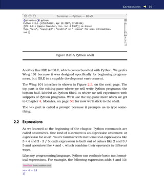
![STYLE NOTES 34
Another is round, which rounds a floating-point number to the nearest
integer:
Download basic/round.cmd
>>> round(3.8)
4.0
>>> round(3.3)
3.0
>>> round(3.5)
4.0
Just like user-defined functions, Python’s built-in functions can take
more than one argument. For example, we can calculate 24
using the
power function pow:
Download basic/two_args.cmd
>>> pow(2, 4)
16
Some of the most useful built-in functions are ones that convert from
one type to another. The type names int and float can be used as if they
were functions:
Download basic/typeconvert.cmd
>>> int(34.6)
34
>>> float(21)
21.0
In this example, we see that when a floating-point number is converted
to an integer and truncated, not rounded.
2.8 Style Notes
Psychologists have discovered that people can keep track of only a
handful of things at any one time [Hoc04]. Since programs can get quite
complicated, it’s important that you choose names for your variables
that will help you remember what they’re for. X1, X2, and blah won’t
remind you of anything when you come back to look at your program
next week; use names like celsius, average, and final_result instead.
Other studies have shown that your brain automatically notices differ-
ences between things—in fact, there’s no way to stop it from doing this.
As a result, the more inconsistencies there are in a piece of text, the
longer it takes to read. (JuSt thInK a bout how long It w o u l d tAKE
you to rEa d this cHaPTer iF IT wAs fORmaTTeD like thIs.) It’s therefore
Report erratum
this copy is (P1.0 printing, April 2009)
Prepared exclusively for Trieu Nguyen](/p?url=https%3A%2F%2Fimage.slidesharecdn.com%2Fpracticalprogramming-230513080735-b837caa3%2F85%2FPractical-Programming-pdf-34-320.jpg&__src=https%3A%2F%2Fwww.slideshare.net%2Fslideshow%2Fpractical-programmingpdf%2F257812881&__type=image)


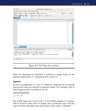
![DEFINING YOUR OWN MODULES 55
The __builtins__ Module
Python’s built-in functions are actually in a module named
__builtins__. The double underscores before and after the name
signal that it’s part of Python; we’ll see this convention used
again later for other things. You can see what’s in the module
using help(__builtins__), or if you just want a directory, you can use
dir instead (which works on other modules as well):
Download modules/dir1.cmd
>>> dir(__builtins__)
['ArithmeticError', 'AssertionError', 'AttributeError',
'BaseException', 'DeprecationWarning', 'EOFError', 'Ellipsis',
'EnvironmentError', 'Exception', 'False', 'FloatingPointError',
'FutureWarning', 'GeneratorExit', 'IOError', 'ImportError',
'ImportWarning', 'IndentationError', 'IndexError', 'KeyError',
'KeyboardInterrupt', 'LookupError', 'MemoryError', 'NameError',
'None', 'NotImplemented', 'NotImplementedError', 'OSError',
'OverflowError', 'PendingDeprecationWarning', 'ReferenceError',
'RuntimeError', 'RuntimeWarning', 'StandardError',
'StopIteration', 'SyntaxError', 'SyntaxWarning', 'SystemError',
'SystemExit', 'TabError', 'True', 'TypeError',
'UnboundLocalError', 'UnicodeDecodeError', 'UnicodeEncodeError',
'UnicodeError', 'UnicodeTranslateError', 'UnicodeWarning',
'UserWarning', 'ValueError', 'Warning', 'ZeroDivisionError', '_',
'__debug__', '__doc__', '__import__', '__name__', 'abs', 'all',
'any', 'apply', 'basestring', 'bool', 'buffer', 'callable',
'chr', 'classmethod', 'cmp', 'coerce', 'compile', 'complex',
'copyright', 'credits', 'delattr', 'dict', 'dir', 'divmod',
'enumerate', 'eval', 'execfile', 'exit', 'file', 'filter',
'float', 'frozenset', 'getattr', 'globals', 'hasattr', 'hash',
'help', 'hex', 'id', 'input', 'int', 'intern', 'isinstance',
'issubclass', 'iter', 'len', 'license', 'list', 'locals', 'long',
'map', 'max', 'min', 'object', 'oct', 'open', 'ord', 'pow',
'property', 'quit', 'range', 'raw_input', 'reduce', 'reload',
'repr', 'reversed', 'round', 'set', 'setattr', 'slice', 'sorted',
'staticmethod', 'str', 'sum', 'super', 'tuple', 'type', 'unichr',
'unicode', 'vars', 'xrange', 'zip']
As of Python 2.5, 32 of the 135 things in __builtins__ are used to
signal errors of particular kinds, such as SyntaxError and ZeroDi-
visionError. There are also functions called copyright, which tells
you who holds the copyright on Python, and license, which dis-
plays Python’s rather complicated license. We’ll meet some of
this module’s other members in later chapters.
Report erratum
this copy is (P1.0 printing, April 2009)
Prepared exclusively for Trieu Nguyen](/p?url=https%3A%2F%2Fimage.slidesharecdn.com%2Fpracticalprogramming-230513080735-b837caa3%2F85%2FPractical-Programming-pdf-55-320.jpg&__src=https%3A%2F%2Fwww.slideshare.net%2Fslideshow%2Fpractical-programmingpdf%2F257812881&__type=image)


![DEFINING YOUR OWN MODULES 58
The same thing happens if we write a program that does nothing but
import our echoing module:
Download modules/import_echo.py
import echo
print "After import, __name__ is", __name__, "and echo.__name__ is", echo.__name__
which, when run from the command line, produces this:
Download modules/import_echo.out
echo: __name__ is echo
After import, __name__ is __main__ and echo.__name__ is echo
What’s happening here is that when Python imports a module, it sets
that module’s __name__ variable to be the name of the module, rather
than the special string "__main__". This means that a module can tell
whether it is the main program:
Download modules/test_main.py
if __name__ == "__main__":
print "I am the main program"
else:
print "Someone is importing me"
Try it, and see what happens when you run it directly and when you
import it.
Knowing whether a module is being imported or not turns out to allow a
few handy programming tricks. One is to provide help on the command
line whenever someone tries to run a module that’s meant to be used
as a library. For example, think about what happens when you run the
following on the command line vs. importing it into another program:
Download modules/main_help.py
'''
This module guesses whether something is a dinosaur or not.
'''
def is_dinosaur(name):
'''
Return True if the named create is recognized as a dinosaur,
and False otherwise.
'''
return name in ['Tyrannosaurus', 'Triceratops']
if __name__ == '__main__':
help(__name__)
We will see other uses in the following sections and in later chapters.
Report erratum
this copy is (P1.0 printing, April 2009)
Prepared exclusively for Trieu Nguyen](/p?url=https%3A%2F%2Fimage.slidesharecdn.com%2Fpracticalprogramming-230513080735-b837caa3%2F85%2FPractical-Programming-pdf-58-320.jpg&__src=https%3A%2F%2Fwww.slideshare.net%2Fslideshow%2Fpractical-programmingpdf%2F257812881&__type=image)


![OBJECTS AND METHODS 63
'Computer Science'.swapcase().endswith('ENCE')
.endswith('ENCE')
'cOMPUTER sCIENCE'
True
Figure 4.4: Chaining method calls
Download modules/swap_endswith.cmd
>>> 'Computer Science'.swapcase().endswith('ENCE')
True
In Figure 4.4, we can see what’s going on when we do this. Note that
Python automatically creates a temporary variable to hold the value of
the swapcase method call long enough for it to call that value’s endswith
method.
Something that has methods is called an object. It turns out that every-
thing in Python is an object, even the number zero:
Download modules/int_help.cmd
>>> help(0)
Help on int object:
class int(object)
| int(x[, base]) -> integer
|
| Convert a string or number to an integer, if possible. A floating point
| argument will be truncated towards zero (this does not include a string
| representation of a floating point number!) When converting a string, use
| the optional base. It is an error to supply a base when converting a
| non-string. If the argument is outside the integer range a long object
| will be returned instead.
|
| Methods defined here:
|
| __abs__(...)
| x.__abs__() <==> abs(x)
|
| __add__(...)
| x.__add__(y) <==> x+y
...
Report erratum
this copy is (P1.0 printing, April 2009)
Prepared exclusively for Trieu Nguyen](/p?url=https%3A%2F%2Fimage.slidesharecdn.com%2Fpracticalprogramming-230513080735-b837caa3%2F85%2FPractical-Programming-pdf-63-320.jpg&__src=https%3A%2F%2Fwww.slideshare.net%2Fslideshow%2Fpractical-programmingpdf%2F257812881&__type=image)


![Chapter 5
Lists
Up to this point, each variable we have created has referred to a single
number or string. In this chapter, we will work with collections of data
and use a Python type named list. Lists contain 0 or more objects, and
they allow us to store data such as 90 experiment measurements or
10,000 student IDs. We’ll also see how to access files and represent
their contents using lists.
5.1 Lists and Indices
Figure 5.1, on the next page, taken from http://www.acschannelislands.
org/2008CountDaily.pdf, shows the number of gray whales counted near
the Coal Oil Point Natural Reserve in a two-week period in the spring of
2008.
Using what we have seen so far, we would have to create fourteen vari-
ables to keep track of these numbers (see Figure 5.2, on the following
page). If we wanted to track an entire year’s worth of observations, we’d
need 366 (just in case it was a leap year). Even worse, if we didn’t know
in advance how long we wanted to watch the whales, we wouldn’t know
how many variables to create.
The solution is to store all the values together in a list. Lists show up
everywhere in the real world: students in a class, the kinds of birds
native to New Guinea, and so on. To create a list in Python, we put the
values, separated by commas, inside square brackets:
Download lists/whalelist.py
# Number of whales seen per day
[5, 4, 7, 3, 2, 3, 2, 6, 4, 2, 1, 7, 1, 3]
Prepared exclusively for Trieu Nguyen](/p?url=https%3A%2F%2Fimage.slidesharecdn.com%2Fpracticalprogramming-230513080735-b837caa3%2F85%2FPractical-Programming-pdf-81-320.jpg&__src=https%3A%2F%2Fwww.slideshare.net%2Fslideshow%2Fpractical-programmingpdf%2F257812881&__type=image)

![LISTS AND INDICES 83
0 1 2 3
5 4 7 3
whales
4 5 6 7
2 3 2 6
8 9 10 11
4 2 1 7
12 13
1 3
Figure 5.3: List example
A list is an object; like any other object, it can be assigned to a variable:
Download lists/whales1.cmd
>>> whales = [5, 4, 7, 3, 2, 3, 2, 6, 4, 2, 1, 7, 1, 3]
>>> whales
[5, 4, 7, 3, 2, 3, 2, 6, 4, 2, 1, 7, 1, 3]
In Figure 5.3, we can see a memory model of whales after this assign-
ment. It’s important to keep in mind that the list itself is one object but
may contain references to other objects (shown by the arrows).
So, how do we get at the objects in a list? By providing an index that
specifies the one we want. The first item in a list is at index 0, the
second at index 1, and so on.1
To refer to a particular item, we put the
index in square brackets after a reference to the list (such as the name
of a variable):
Download lists/whales2.cmd
>>> whales = [5, 4, 7, 3, 2, 3, 2, 6, 4, 2, 1, 7, 1, 3]
>>> whales[0]
5
>>> whales[1]
4
>>> whales[12]
1
>>> whales[13]
3
We can use only those indices that are in the range from zero up to one
less than the length of the list. In a fourteen-item list, the legal indices
are 0, 1, 2, and so on, up to 13. Trying to use an out-of-range index is
an error, just like trying to divide by zero.
1. Yes, it would be more natural to use 1 as the first index, as human languages do.
Python, however, uses the same convention as languages like C and Java and starts
counting at zero.
Report erratum
this copy is (P1.0 printing, April 2009)
Prepared exclusively for Trieu Nguyen](/p?url=https%3A%2F%2Fimage.slidesharecdn.com%2Fpracticalprogramming-230513080735-b837caa3%2F85%2FPractical-Programming-pdf-83-320.jpg&__src=https%3A%2F%2Fwww.slideshare.net%2Fslideshow%2Fpractical-programmingpdf%2F257812881&__type=image)
![LISTS AND INDICES 84
Download lists/whales3.cmd
>>> whales = [5, 4, 7, 3, 2, 3, 2, 6, 4, 2, 1, 7, 1, 3]
>>> whales[1001]
Traceback (most recent call last):
File "<stdin>", line 1, in ?
IndexError: list index out of range
Unlike most programming languages, Python also lets us index back-
ward from the end of a list. The last item is at index -1, the one before
it at index -2, and so on:
Download lists/whales4.cmd
>>> whales = [5, 4, 7, 3, 2, 3, 2, 6, 4, 2, 1, 7, 1, 3]
>>> whales[-1]
3
>>> whales[-2]
1
>>> whales[-14]
5
We can assign the values in a list to other variables:
Download lists/whales5.cmd
>>> whales = [5, 4, 7, 3, 2, 3, 2, 6, 4, 2, 1, 7, 1, 3]
>>> third = whales[2]
>>> print 'Third day:', third
Third day: 7
The Empty List
Zero is a useful number, and as we saw in Chapter 3, Strings, on
page 39, the empty string is often useful as well. There is also an empty
list, in other words, a list with no items in it. As you might guess, it is
written [ ]. Trying to index an empty list always results in an error:
Download lists/whales6.cmd
>>> whales = []
>>> whales[0]
Traceback (most recent call last):
File "<stdin>", line 1, in <module>
IndexError: list index out of range
>>> whales[-1]
Traceback (most recent call last):
File "<stdin>", line 1, in <module>
IndexError: list index out of range
Report erratum
this copy is (P1.0 printing, April 2009)
Prepared exclusively for Trieu Nguyen](/p?url=https%3A%2F%2Fimage.slidesharecdn.com%2Fpracticalprogramming-230513080735-b837caa3%2F85%2FPractical-Programming-pdf-84-320.jpg&__src=https%3A%2F%2Fwww.slideshare.net%2Fslideshow%2Fpractical-programmingpdf%2F257812881&__type=image)
![MODIFYING LISTS 85
This follows from the definition of legal index:
• Legal indices for a list of N items are the integers in the set {i: 0 ≤
i < N}.
• The length of the empty list is 0.
• Legal indices for the empty list are therefore the elements of the
set {i: 0 ≤ i < -1}.
• Since this set is empty, there are no legal indices for the empty
list.
Lists Are Heterogeneous
Lists can contain any type of data, including integers, strings, and even
other lists. Here is a list of information about the element Krypton,
including its name, symbol, melting point (in degrees Celsius), and
boiling point (also in degrees Celsius). Using a list to aggregate related
information is somewhat prone to error; a better, but more advanced,
way to do this is described in Chapter 13, Object-Oriented Programming,
on page 270.
Download lists/krypton1.cmd
>>> krypton = ['Krypton', 'Kr', -157.2, -153.4]
>>> krypton[1]
'Kr'
>>> krypton[2]
-157.19999999999999
5.2 Modifying Lists
Suppose we’re typing in a list of the noble gases2
and our fingers slip:
Download lists/nobles1.cmd
>>> nobles = ['helium', 'none', 'argon', 'krypton', 'xenon', 'radon']
The error here is that we typed ’none’ instead of ’neon’. Rather than
retyping the whole list, we can assign a new value to a specific element
of the list:
Download lists/nobles2.cmd
>>> nobles = ['helium', 'none', 'argon', 'krypton', 'xenon', 'radon']
>>> nobles[1] = 'neon'
>>> nobles
['helium', 'neon', 'argon', 'krypton', 'xenon', 'radon']
2. A noble gas is one whose outermost electron shell is completely full, which makes it
chemically inert.
Report erratum
this copy is (P1.0 printing, April 2009)
Prepared exclusively for Trieu Nguyen](/p?url=https%3A%2F%2Fimage.slidesharecdn.com%2Fpracticalprogramming-230513080735-b837caa3%2F85%2FPractical-Programming-pdf-85-320.jpg&__src=https%3A%2F%2Fwww.slideshare.net%2Fslideshow%2Fpractical-programmingpdf%2F257812881&__type=image)
![BUILT -IN FUNCTIONS ON LISTS 86
0 1 2 3
'helium' 'none' 'argon' 'krypton'
nobles
4
'xenon'
Before
5
'radon'
After
0 1 2 3
'helium' 'none' 'argon' 'krypton'
nobles
4
'xenon'
5
'radon'
'neon'
Figure 5.4: List mutation
In Figure 5.4, we show what the assignment to nobles[1] did. It also
shows that lists are mutable, in other words, that their contents can be
changed after they have been created. In contrast, numbers and strings
are immutable. You cannot, for example, change a letter in a string after
you have created it. Methods that appear to, like upper, actually create
new strings:
Download lists/strings_immutable.cmd
>>> name = 'Darwin'
>>> capitalized = name.upper()
>>> print capitalized
'DARWIN'
>>> print name
'Darwin'
The expression L[i] behaves just like a simple variable (see Section 2.4,
Variables and the Assignment Statement, on page 25). If it’s on the right,
it means “Get the value of the item at location i in the list L.” If it’s on
the left, it means “Figure out where item i in the list L is located so that
we can overwrite it.”
Report erratum
this copy is (P1.0 printing, April 2009)
Prepared exclusively for Trieu Nguyen](/p?url=https%3A%2F%2Fimage.slidesharecdn.com%2Fpracticalprogramming-230513080735-b837caa3%2F85%2FPractical-Programming-pdf-86-320.jpg&__src=https%3A%2F%2Fwww.slideshare.net%2Fslideshow%2Fpractical-programmingpdf%2F257812881&__type=image)
![BUILT -IN FUNCTIONS ON LISTS 87
Function Description
len(L) Returns the number of items in list L
max(L) Returns the maximum value in list L
min(L) Returns the minimum value in list L
sum(L) Returns the sum of the values in list L
Figure 5.5: List functions
5.3 Built-in Functions on Lists
Section 2.6, Function Basics, on page 30 introduced a few of Python’s
built-in functions. Some of these, such as len, can be applied to lists as
well, as can others that we haven’t seen before (see Figure 5.5). Here
they are in action working on a list of the half-lives3
of our plutonium
isotopes:
Download lists/plu4.cmd
>>> half_lives = [87.74, 24110.0, 6537.0, 14.4, 376000.0]
>>> len(half_lives)
5
>>> max(half_lives)
376000.0
>>> min(half_lives)
14.4
>>> sum(half_lives)
406749.14000000001
We can use the results of the built-in functions in expressions; for
example, the following code demonstrates that we can check whether
an index is in range:
Download lists/plu5.cmd
>>> half_lives = [87.74, 24110.0, 6537.0, 14.4, 376000.0]
>>> i = 2
>>> 0 <= i < len(half_lives)
True
>>> half_lives[i]
6537.0
>>> i = 5
>>> 0 <= i < len(half_lives)
False
3. The half-life of a radioactive substance is the time taken for half of it to decay. After
twice this time has gone by, three quarters of the material will have decayed; after three
times, seven eighths, and so on.
Report erratum
this copy is (P1.0 printing, April 2009)
Prepared exclusively for Trieu Nguyen](/p?url=https%3A%2F%2Fimage.slidesharecdn.com%2Fpracticalprogramming-230513080735-b837caa3%2F85%2FPractical-Programming-pdf-87-320.jpg&__src=https%3A%2F%2Fwww.slideshare.net%2Fslideshow%2Fpractical-programmingpdf%2F257812881&__type=image)
![BUILT -IN FUNCTIONS ON LISTS 88
0 1 2 3
0 1
'H' 'He'
original
final
2
'Li'
0
'Be'
Figure 5.6: List concatenation
>>> half_lives[i]
Traceback (most recent call last):
File "<stdin>", line 1, in ?
IndexError: list index out of range
Like all other objects, lists have a particular type, and Python complains
if you try to combine types in inappropriate ways. Here’s what happens
if you try to “add” a list and a string:
Download lists/add_list_str.cmd
>>> ['H', 'He', 'Li'] + 'Be'
Traceback (most recent call last):
File "<stdin>", line 1, in <module>
TypeError: can only concatenate list (not "str") to list
That error report is interesting. It hints that we might be able to con-
catenate lists with lists to create new lists, just as we concatenated
strings to create new strings. A little experimentation shows that this
does in fact work:
Download lists/concat_lists.cmd
>>> original = ['H', 'He', 'Li']
>>> final = original + ['Be']
>>> final
['H', 'He', 'Li', 'Be']
As shown in Figure 5.6, this doesn’t modify either of the original lists.
Instead, it creates a new list whose entries refer to the entries of the
original lists.
Report erratum
this copy is (P1.0 printing, April 2009)
Prepared exclusively for Trieu Nguyen](/p?url=https%3A%2F%2Fimage.slidesharecdn.com%2Fpracticalprogramming-230513080735-b837caa3%2F85%2FPractical-Programming-pdf-88-320.jpg&__src=https%3A%2F%2Fwww.slideshare.net%2Fslideshow%2Fpractical-programmingpdf%2F257812881&__type=image)
![PROCESSING LIST ITEMS 89
So if + works on lists, will sum work on lists of strings? After all, if sum([1,
2, 3]) is the same as 1 + 2 + 3, shouldn’t sum(’a’, ’b’, ’c’) be the same as
’a’ + ’b’ + ’c’, or ’abc’? The following code shows that the analogy can’t
be pushed that far:
Download lists/sum_of_str.cmd
>>> sum(['a', 'b', 'c'])
Traceback (most recent call last):
File "<stdin>", line 1, in <module>
TypeError: unsupported operand type(s) for +: 'int' and 'str'
On the other hand, you can multiply a list by an integer to get a new
list containing the elements from the original list repeated a certain
number of times:
Download lists/mult_lists.cmd
>>> metals = 'Fe Ni'.split()
>>> metals * 3
['Fe', 'Ni', 'Fe', 'Ni', 'Fe', 'Ni']
As with concatenation, the original list isn’t modified; instead, a new
list is created. Notice, by the way, how we use string.split to turn the
string ’Fe Ni’ into a two-element list [’Fe’, ’Ni’]. This is a common trick in
Python programs.
5.4 Processing List Items
Lists were invented so that we wouldn’t have to create 1,000 variables
to store a thousand values. For the same reason, Python has a for loop
that lets us process each element in a list in turn, without having to
write one statement per element. The general form of a for loop is as
follows:
for variable in list:
block
As we saw in Section 2.6, Function Basics, on page 30, a block is just a
sequence of one or more statements. variable and list are just a variable
and a list.
When Python encounters a loop, it executes the loop’s block once for
each value in the list. Each pass through the block is called an iteration,
and at the start of each iteration, Python assigns the next value in the
list to the specified variable. In this way, the program can do something
with each value in turn.
Report erratum
this copy is (P1.0 printing, April 2009)
Prepared exclusively for Trieu Nguyen](/p?url=https%3A%2F%2Fimage.slidesharecdn.com%2Fpracticalprogramming-230513080735-b837caa3%2F85%2FPractical-Programming-pdf-89-320.jpg&__src=https%3A%2F%2Fwww.slideshare.net%2Fslideshow%2Fpractical-programmingpdf%2F257812881&__type=image)
![PROCESSING LIST ITEMS 90
For example, this code prints every velocity of a falling object in metric
and imperial units:
Download lists/velocity_loop.cmd
>>> velocities = [0.0, 9.81, 19.62, 29.43]
>>> for v in velocities:
... print "Metric:", v, "m/sec;",
... print "Imperial:", v * 3.28, "ft/sec"
...
Metric: 0.0 m/sec; Imperial: 0.0 ft/sec
Metric: 9.81 m/sec; Imperial: 32.1768 ft/sec
Metric: 19.62 m/sec; Imperial: 64.3536 ft/sec
Metric: 29.43 m/sec; Imperial: 96.5304 ft/sec
Here are two other things to notice about this loop:
• In English we would say “for each velocity in the list, print the
metric value, and then print the imperial value.” In Python, we
said roughly the same thing.
• As with function definitions, the statements in the loop block are
indented. (We use four spaces in this book; check with your in-
structors to find out whether they prefer something else.)
In this case, we created a new variable v to store the current value
taken from the list inside the loop. We could equally well have used an
existing variable. If we do this, the loop still starts with the first element
of the list—whatever value the variable had before the loop is lost:
Download lists/velocity_recycle.cmd
>>> speed = 2
>>> velocities = [0.0, 9.81, 19.62, 29.43]
>>> for speed in velocities:
... print "Metric:", speed, "m/sec;",
...
Metric: 0.0 m/sec
Metric: 9.81 m/sec
Metric: 19.62 m/sec
Metric: 29.43 m/sec
>>> print "Final:", speed
Final: 29.43
Either way, the variable is left holding its last value when the loop fin-
ishes. Notice, by the way, that the last print statement in this program
is not indented, so it is not part of the for loop. It is executed after the
for loop has finished and is executed only once.
Nested Loops
We said earlier that the block of statements inside a loop could contain
anything. This means that it can also contain another loop.
Report erratum
this copy is (P1.0 printing, April 2009)
Prepared exclusively for Trieu Nguyen](/p?url=https%3A%2F%2Fimage.slidesharecdn.com%2Fpracticalprogramming-230513080735-b837caa3%2F85%2FPractical-Programming-pdf-90-320.jpg&__src=https%3A%2F%2Fwww.slideshare.net%2Fslideshow%2Fpractical-programmingpdf%2F257812881&__type=image)
![PROCESSING LIST ITEMS 91
This program, for example, loops over the list inner once for each ele-
ment of the list outer:
Download lists/nested_loops.cmd
>>> outer = ['Li', 'Na', 'K']
>>> inner = ['F', 'Cl', 'Br']
>>> for metal in outer:
... for gas in inner:
... print metal + gas
...
...
LiF
LiCl
LiBr
NaF
NaCl
NaBr
KF
KCl
KBr
If the outer loop has No iterations and the inner loop executes Ni times
for each of them, the inner loop will execute a total of NoNi times. One
special case of this is when the inner and outer loops are running over
the same list of length N, in which case the inner loop executes N2
times.
This can be used to generate a multiplication table; after printing the
header row, we use a nested loop to print each row of the table in turn,
using tabs to make the columns line up:
Download lists/multiplication_table.py
def print_table():
'''Print the multiplication table for numbers 1 through 5.'''
numbers = [1, 2, 3, 4, 5]
# Print the header row.
for i in numbers:
print 't' + str(i),
print # End the header row.
# Print the column number and the contents of the table.
for i in numbers:
print i,
for j in numbers:
print 't' + str(i * j),
print # End the current row.
Report erratum
this copy is (P1.0 printing, April 2009)
Prepared exclusively for Trieu Nguyen](/p?url=https%3A%2F%2Fimage.slidesharecdn.com%2Fpracticalprogramming-230513080735-b837caa3%2F85%2FPractical-Programming-pdf-91-320.jpg&__src=https%3A%2F%2Fwww.slideshare.net%2Fslideshow%2Fpractical-programmingpdf%2F257812881&__type=image)
![SLICING 92
Here is print_table’s output:
Download lists/multiplication_out.txt
>>> from multiplication_table import *
>>> print_table()
1 2 3 4 5
1 1 2 3 4 5
2 2 4 6 8 10
3 3 6 9 12 15
4 4 8 12 16 20
5 5 10 15 20 25
Notice when the two different kinds of formatting are done: the print
statement at the bottom of the program prints a new line when outer
loop advances, while the inner loop includes a tab in front of each item.
5.5 Slicing
Geneticists describe C. elegans (nematodes, or microscopic worms)
using three-letter short-form markers. Examples include Emb (embry-
onic lethality), Him (High incidence of males), Unc (Uncoordinated), Dpy
(dumpy: short and fat), Sma (small), and Lon (long). We can thus keep
a list:
Download lists/celegans.cmd
>>> celegans_markers = ['Emb', 'Him', 'Unc', 'Lon', 'Dpy', 'Sma']
>>> celegans_markers
['Emb', 'Him', 'Unc', 'Lon', 'Dpy', 'Sma']
It turns out that Dpy worms and Sma worms are difficult to distin-
guish from each other, so they are not as useful as markers in complex
strains. We can produce a new list based on celegans_markers, but with-
out Dpy or Sma, by taking a slice of the list:
Download lists/celegans1.cmd
>>> celegans_markers = ['Emb', 'Him', 'Unc', 'Lon', 'Dpy', 'Sma']
>>> useful_markers = celegans_markers[0:4]
This creates a new list consisting of only the four distinguishable mark-
ers (see Figure 5.7, on the following page).
The first index in the slice is the starting point. The second index is one
more than the index of the last item we want to include. More rigorously,
Report erratum
this copy is (P1.0 printing, April 2009)
Prepared exclusively for Trieu Nguyen](/p?url=https%3A%2F%2Fimage.slidesharecdn.com%2Fpracticalprogramming-230513080735-b837caa3%2F85%2FPractical-Programming-pdf-92-320.jpg&__src=https%3A%2F%2Fwww.slideshare.net%2Fslideshow%2Fpractical-programmingpdf%2F257812881&__type=image)
![SLICING 93
0 1 2 3
'Emb' 'Him' 'Unc' 'Lon'
celegans_markers
'Dpy'
4
1
useful_markers
0
'Sma'
5
3
2
Figure 5.7: Slicing doesn’t modify lists.
list[i:j] is a slice of the original list from index i (inclusive) up to, but not
including, index j (exclusive).4
The first index can be omitted if we want to slice from the beginning of
the list, and the last index can be omitted if we want to slice to the end:
Download lists/celegans2.cmd
>>> celegans_markers = ['Emb', 'Him', 'Unc', 'Lon', 'Dpy', 'Sma']
>>> celegans_markers[:4]
['Emb', 'Him', 'Unc', 'Lon']
>>> celegans_markers[4:]
['Dpy', 'Sma']
To create a copy of the entire list, we just omit both indices so that the
“slice” runs from the start of the list to its end:
Download lists/celegans3.cmd
>>> celegans_markers = ['Emb', 'Him', 'Unc', 'Lon', 'Dpy', 'Sma']
>>> celegans_copy = celegans_markers[:]
>>> celegans_markers[5] = 'Lvl'
>>> celegans_markers
['Emb', 'Him', 'Unc', 'Lon', 'Dpy', 'Lvl']
>>> celegans_copy
['Emb', 'Him', 'Unc', 'Lon', 'Dpy', 'Sma']
4. Python uses this convention to be consistent with the rule that the legal indices for a
list go from 0 up to one less than the list’s length.
Report erratum
this copy is (P1.0 printing, April 2009)
Prepared exclusively for Trieu Nguyen](/p?url=https%3A%2F%2Fimage.slidesharecdn.com%2Fpracticalprogramming-230513080735-b837caa3%2F85%2FPractical-Programming-pdf-93-320.jpg&__src=https%3A%2F%2Fwww.slideshare.net%2Fslideshow%2Fpractical-programmingpdf%2F257812881&__type=image)
![ALIASING 94
0 1 2 3
'Emb' 'Him' 'Unc' 'Lon'
celegans_markers
'Dpy'
4
'Sma'
5
celegans_copy
Figure 5.8: Aliasing lists
5.6 Aliasing
An alias is an alternative name for something. In Python, two variables
are said to be aliases when they refer to the same value. For example,
the following code creates two variables, both of which refer to a single
list (see Figure 5.8). When we modify the list using one of the variables,
references through the other variable show the change as well:
Download lists/celegans4.cmd
>>> celegans_markers = ['Emb', 'Him', 'Unc', 'Lon', 'Dpy', 'Sma']
>>> celegans_copy = celegans_markers
>>> celegans_markers[5] = 'Lvl'
>>> celegans_markers
['Emb', 'Him', 'Unc', 'Lon', 'Dpy', 'Lvl']
>>> celegans_copy
['Emb', 'Him', 'Unc', 'Lon', 'Dpy', 'Lvl']
Aliasing is one of the reasons why the notion of mutability is important.
For example, if x and y refer to the same list, then any changes you
make to the list through x will be “seen” by y, and vice versa. This can
lead to all sorts of hard-to-find errors in which a list’s value changes
as if by magic, even though your program doesn’t appear to assign
anything to it. This can’t happen with immutable values like strings.
Since a string can’t be changed after it has been created, it’s safe to
have aliases for it.
Aliasing in Function Calls
Aliasing occurs when we use list parameters as well, since parameters
are variables.
Report erratum
this copy is (P1.0 printing, April 2009)
Prepared exclusively for Trieu Nguyen](/p?url=https%3A%2F%2Fimage.slidesharecdn.com%2Fpracticalprogramming-230513080735-b837caa3%2F85%2FPractical-Programming-pdf-94-320.jpg&__src=https%3A%2F%2Fwww.slideshare.net%2Fslideshow%2Fpractical-programmingpdf%2F257812881&__type=image)
![LIST METHODS 95
Method Description
L.append(v) Appends value v to list L
L.insert(i, v) Inserts value v at index i in list L, shifting following items
to make room
L.remove(v) Removes the first occurrence of value v from list L
L.reverse() Reverses the order of the values in list L
L.sort() Sorts the values in list L in ascending order (for strings,
alphabetical order)
L.pop() Removes and returns the last element of L (which must be
nonempty)
Figure 5.9: List methods
Here is a simple function that takes a list, sorts it, and then reverses it:
Download lists/alias_parameters.cmd
>>> def sort_and_reverse(L):
... '''Return list L sorted and reversed.'''
... L.sort()
... L.reverse()
... return L
...
>>> celegans_markers = ['Emb', 'Him', 'Unc', 'Lon', 'Dpy', 'Lvl']
>>> sort_and_reverse(celegans_markers)
['Unc', 'Lvl', 'Lon', 'Him', 'Emb', 'Dpy']
>>> celegans_markers
['Unc', 'Lvl', 'Lon', 'Him', 'Emb', 'Dpy']
This function modifies list L, and since L is an alias of celegans_markers,
that list is modified as well.
5.7 List Methods
Lists are objects and thus have methods. Some of the most commonly
used are listed in Figure 5.9. Here is a sample interaction showing how
we can use these methods to construct a list containing all the colors
of the rainbow:
Download lists/colors.cmd
>>> colors = 'red orange green black blue'.split()
>>> colors.append('purple')
>>> colors
['red', 'orange', 'green', 'black', 'blue', 'purple']
Report erratum
this copy is (P1.0 printing, April 2009)
Prepared exclusively for Trieu Nguyen](/p?url=https%3A%2F%2Fimage.slidesharecdn.com%2Fpracticalprogramming-230513080735-b837caa3%2F85%2FPractical-Programming-pdf-95-320.jpg&__src=https%3A%2F%2Fwww.slideshare.net%2Fslideshow%2Fpractical-programmingpdf%2F257812881&__type=image)
![LIST METHODS 96
Where Did My List Go?
Beginning programmers often forget that many list methods
return None rather than creating and returning a new list. (Expe-
rienced programmers sometimes forget too.) As a result, their
lists sometimes seem to disappear:
Download lists/colors2.cmd
>>> colors = 'red orange yellow green blue purple'.split()
>>> colors
['blue', 'green', 'orange', 'purple', 'red', 'yellow']
>>> sorted_colors = colors.sort()
>>> print sorted_colors
None
As we’ll discuss in Section 4.5, Testing, on page 70, mistakes like
these can quickly be caught by writing and running a few tests.
>>> colors.insert(2, 'yellow')
>>> colors
['red', 'orange', 'yellow', 'green', 'black', 'blue', 'black', 'purple']
>>> colors.remove('black')
>>> colors
['red', 'orange', 'yellow', 'green', 'blue', 'purple']
It is important to note that all these methods modify the list instead
of creating a new list. They do this because lists can grow very, very
large—a million patient records, for example, or a billion measurements
of a magnetic field. Creating a new list every time someone wanted to
make a change to such a list would slow Python down so much that it
would no longer be useful; having Python guess when it should make
a copy, and when it should operate on the list in place, would make it
impossible to figure out.
It’s just as important to remember that all of these methods except
pop return the special value None, which means “There is no useful
information” or “There’s nothing here.” Python doesn’t display anything
when asked to display the value None. Printing it, on the other hand,
shows us that it’s there:
Download lists/none.cmd
>>> x = None
>>> x
>>> print x
None
Report erratum
this copy is (P1.0 printing, April 2009)
Prepared exclusively for Trieu Nguyen](/p?url=https%3A%2F%2Fimage.slidesharecdn.com%2Fpracticalprogramming-230513080735-b837caa3%2F85%2FPractical-Programming-pdf-96-320.jpg&__src=https%3A%2F%2Fwww.slideshare.net%2Fslideshow%2Fpractical-programmingpdf%2F257812881&__type=image)
![NESTED LISTS 97
0
life
1 2
0 1 0 1 0 1
'Canada' 80
'United States' 75.5
'Mexico' 72.0
Figure 5.10: Nested lists
Finally, a call to append is not the same as using +. First, append
appends a single value, while + expects two lists as operands. Second,
append modifies the list rather than creating a new one.
5.8 Nested Lists
We said in Section 5.1, Lists Are Heterogeneous, on page 85 that lists
can contain any type of data. That means that they can contain other
lists, just as the body of a loop can contain another loop. For example,
the following nested list describes life expectancies in different coun-
tries:
Download lists/lifelist.py
[['Canada', 76.5], ['United States', 75.5], ['Mexico', 72.0]]
As shown in Figure 5.10, each element of the outer list is itself a list
of two items. We use the standard notation to access the items in the
outer list:
Download lists/life0.cmd
>>> life = [['Canada', 76.5], ['United States', 75.5], ['Mexico', 72.0]]
>>> life[0]
['Canada', 76.5]
>>> life[1]
['United States', 75.5]
>>> life[2]
['Mexico', 72.0]
Report erratum
this copy is (P1.0 printing, April 2009)
Prepared exclusively for Trieu Nguyen](/p?url=https%3A%2F%2Fimage.slidesharecdn.com%2Fpracticalprogramming-230513080735-b837caa3%2F85%2FPractical-Programming-pdf-97-320.jpg&__src=https%3A%2F%2Fwww.slideshare.net%2Fslideshow%2Fpractical-programmingpdf%2F257812881&__type=image)
![NESTED LISTS 98
0
life
1 2
0 1 0 1 0 1
'Canada' 76.5
'United States' 75.5
'Mexico' 72.0
canada
Figure 5.11: Aliasing sublists
Since each of these items is also a list, we can immediately index it
again, just as we can chain together method calls or pass the result of
one function call as an argument to another function:
Download lists/life1.cmd
>>> life = [['Canada', 76.5], ['United States', 75.5], ['Mexico', 72.0]]
>>> life[1]
['United States', 75.5]
>>> life[1][0]
'United States'
>>> life[1][1]
75.5
We can also assign sublists to variables:
Download lists/life2.cmd
>>> life = [['Canada', 76.5], ['United States', 75.5], ['Mexico', 72.0]]
>>> canada = life[0]
>>> canada
['Canada', 76.5]
>>> canada[0]
'Canada'
>>> canada[1]
76.5
Assigning a sublist to a variable creates an alias for that sublist (see
Figure 5.11). As before, any change we make through the sublist refer-
ence will show up when we access the main list, and vice versa:
Download lists/life3.cmd
>>> life = [['Canada', 76.5], ['United States', 75.5], ['Mexico', 72.0]]
>>> canada = life[0]
Report erratum
this copy is (P1.0 printing, April 2009)
Prepared exclusively for Trieu Nguyen](/p?url=https%3A%2F%2Fimage.slidesharecdn.com%2Fpracticalprogramming-230513080735-b837caa3%2F85%2FPractical-Programming-pdf-98-320.jpg&__src=https%3A%2F%2Fwww.slideshare.net%2Fslideshow%2Fpractical-programmingpdf%2F257812881&__type=image)
![OTHER KINDS OF SEQUENCES 99
>>> canada[1] = 80.0
>>> canada
['Canada', 80.0]
>>> life
[['Canada', 80.0], ['United States', 75.5], ['Mexico', 72.0]]
5.9 Other Kinds of Sequences
Lists aren’t the only kind of sequence in Python. You’ve already met one
of the others: strings. Formally, a string is an immutable sequence of
characters. The “sequence” part of this definition means that it can be
indexed and sliced like a list to create new strings:
Download lists/string_seq.cmd
>>> rock = 'anthracite'
>>> rock[9]
'e'
>>> rock[0:3]
'ant'
>>> rock[-5:]
'acite'
>>> for character in rock[:5]:
... print character
...
a
n
t
h
r
Python also has an immutable sequence type called a tuple. Tuples are
written using parentheses instead of square brackets; like strings and
lists, they can be subscripted, sliced, and looped over:
Download lists/tuples1.cmd
>>> bases = ('A', 'C', 'G', 'T')
... for b in bases:
... print b
A
C
G
T
There is one small catch: although () represents the empty tuple, a tuple
with one element is not written as (x) but instead as (x,) (with a trailing
comma). This has to be done to avoid ambiguity. If the trailing comma
weren’t required, (5 + 3) could mean either 8 (under the normal rules of
Report erratum
this copy is (P1.0 printing, April 2009)
Prepared exclusively for Trieu Nguyen](/p?url=https%3A%2F%2Fimage.slidesharecdn.com%2Fpracticalprogramming-230513080735-b837caa3%2F85%2FPractical-Programming-pdf-99-320.jpg&__src=https%3A%2F%2Fwww.slideshare.net%2Fslideshow%2Fpractical-programmingpdf%2F257812881&__type=image)
![FILES AS LISTS 100
arithmetic) or the tuple containing only the value 8. This is one of the
few places where Python’s syntax leaves something to be desired....
Once a tuple is created, it cannot be changed:
Download lists/life4.cmd
>>> life = (['Canada', 76.5], ['United States', 75.5], ['Mexico', 72.0])
>>> life[0] = life[1]
Traceback (most recent call last):
File "<stdin>", line 1, in ?
TypeError: object does not support item assignment
However, the objects inside it can still be changed:
Download lists/life5.cmd
>>> life = (['Canada', 76.5], ['United States', 75.5], ['Mexico', 72.0])
>>> life[0][1] = 80.0
>>> life
(['Canada', 80.0], ['United States', 75.5], ['Mexico', 72.0])
This is because it’s actually sloppy English to say that something is
“inside” a tuple. It would be more accurate to say this: “The references
contained in a tuple cannot be changed after the tuple has been cre-
ated, though the objects referred to may themselves change.”
Newcomers to Python often ask why tuples exist. The answer is that
they make some operations more efficient and others safer. We won’t
get far enough in this book to explain the former, but we will explore
the latter in Chapter 9, Sets and Dictionaries, on page 185.
5.10 Files as Lists
Most data is stored in files, which are just ordered sequences of bytes.
Those bytes may represent characters, pixels, or postal codes; the im-
portant thing is that they’re in a particular order, which means that
lists are usually a natural way to work with them.
In order to read data from a file, we must first open it using Python’s
built-in function open:
Download lists/open_basic.cmd
>>> file = open("data.txt", "r")
The first argument to open is a string containing the name of the file.
The second argument indicates a mode. The three options are "r" for
reading, "w" for writing, and "a" for appending. (The difference between
Report erratum
this copy is (P1.0 printing, April 2009)
Prepared exclusively for Trieu Nguyen](/p?url=https%3A%2F%2Fimage.slidesharecdn.com%2Fpracticalprogramming-230513080735-b837caa3%2F85%2FPractical-Programming-pdf-100-320.jpg&__src=https%3A%2F%2Fwww.slideshare.net%2Fslideshow%2Fpractical-programmingpdf%2F257812881&__type=image)