Downloaded 335 times
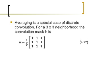
![Averaging with Limited Data
Validity
Methods that average with limited data validity
try to avoid blurring by averaging only those
pixels which satisfy some criterion, the aim
being to prevent involving pixels that are part of
a separate feature.
A very simple criterion is to use only pixels in
the original image with brightness in a
predefined interval of invalid data [min,max].](https://image.slidesharecdn.com/imagepre-processing-localprocessing-121206041411-phpapp01/85/Image-pre-processing-local-processing-16-320.jpg)
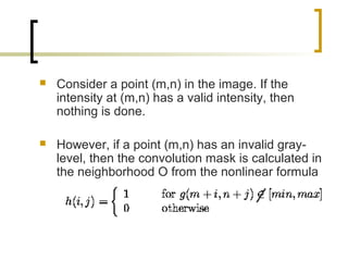


![Averaging with Limited Data
Validity
Methods that average with limited data validity
try to avoid blurring by averaging only those
pixels which satisfy some criterion, the aim
being to prevent involving pixels that are part of
a separate feature.
A very simple criterion is to use only pixels in
the original image with brightness in a
predefined interval of invalid data [min,max].](/p?url=https%3A%2F%2Fimage.slidesharecdn.com%2Fimagepre-processing-localprocessing-121206041411-phpapp01%2F85%2FImage-pre-processing-local-processing-16-320.jpg&__src=https%3A%2F%2Fwww.slideshare.net%2Fslideshow%2Fimage-pre-processing-local-processing%2F15514969%238&__type=image)


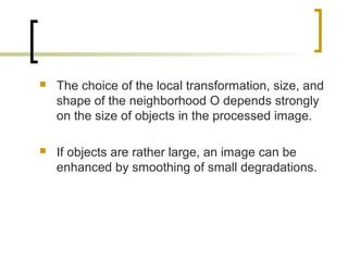
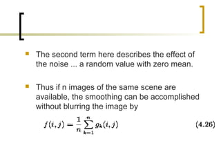
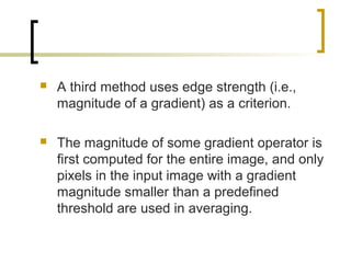
![ If g(m,n) = g(i,j) then we define (i,j,m,n) = 2;
the inverse gradient is then in the interval (0,2],
and is smaller on the edge than in the interior of
a homogeneous region.
Weight coefficients in the convolution mask h are
normalized by the inverse gradient, and the
whole term is multiplied by 0.5 to keep brightness
values in the original range.](/p?url=https%3A%2F%2Fimage.slidesharecdn.com%2Fimagepre-processing-localprocessing-121206041411-phpapp01%2F85%2FImage-pre-processing-local-processing-21-320.jpg&__src=https%3A%2F%2Fwww.slideshare.net%2Fslideshow%2Fimage-pre-processing-local-processing%2F15514969%238&__type=image)


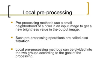
The document discusses various image pre-processing techniques, including: 1) Local pre-processing methods like smoothing and gradient operators that use a neighborhood of pixels to calculate output pixel values. 2) Common smoothing methods include averaging, median filtering, and techniques that average only similar neighboring pixels to reduce blurring. 3) Gradient operators like Roberts, Prewitt, Sobel, and Kirsch detect edges by approximating the image derivative using pixel differences. The Marr-Hildreth technique detects zero-crossings of the second derivative.