ADA complete notes

ANALYSIS AND DESIGN OF ALGORITHMS

SUBJECT CODE: MCA-44

Prepared By:
S.P.Sreeja
Asst. Prof.,
Dept. of MCA
New Horizon College of Engineering

NOTE:

• These notes are intended for use by students in MCA
• These notes are provided free of charge and may not be sold in any shape or form
• These notes are NOT a substitute for material covered during course lectures. If
you miss a lecture, you should definitely obtain both these notes and notes written
by a student who attended the lecture.
• Material from these notes is obtained from various sources, including, but not
limited to, the following:

Text Books:
1. Introduction to Design and Analysis of Algorithms by Anany Levitin, Pearson
Edition, 2003.
Reference Books:
1. Introduction to Algorithms by Coreman T.H., Leiserson C. E., and Rivest R. L.,
PHI, 1998.
2. Computer Algorithms by Horowitz E., Sahani S., and Rajasekharan S., Galgotia
Publications, 2001.

Page No

Chapter 1: INTRODUCTION…………………………………….1

1.1 : Notion of algorithm………………………………..……1
1.2 : Fundamentals of Algorithmic
problem solving..…………………………………...…...3
1.3 : Important problem types…………………………….….6
1.4 : Fundamental data structures……………………..……...9

Chapter 2: FUNDAMENTALS OF THE ANALYSIS OF
ALGORITHM EFFICIENCY………………………..18

2.1 : Analysis Framework……………………………………18
2.2 : Asymptotic Notations and Basic
efficiency classes………………………………………..23
2.3 : Mathematical analysis of
Non recursive algorithms……………………………….29
2.4 : Mathematical analysis of
recursive algorithms……………………………………32
2.5 : Examples……………………………………………….35

Chapter 3: BRUTE FORCE……………………………………..39

3.1 : Selection sort and Bubble sort…………………………39
3.2 : Sequential search Brute Force
string matching…………………………………………43
3.3 : Exhaustive search………………………………………45

Chapter 4: DIVIDE AND CONQUER…………………………..49

4.1 : Merge sort……………………………………………...50
4.2 : Quick sort……………………………………………...53
4.3 : Binary search…………………………………………..57
4.4 : Binary tree traversals and
related properties………………………………………60
4.5 : Multiplication of large integers ……………………….63
4.6 : Strassen’s Matrix Multiplication……………………...65

(i)

Page No

Chapter 5: DECREASE AND CONQUER………………………...67

5.1 : Insertion sort………………………………………………68
5.2 : Depth – First and Breadth – First
search……………………………………………………..71
5.3 : Topological Sorting……………………………………….77
5.4 : Algorithm for Generating
Combinatorial Objects…………………………………….80

Chapter 6: TRANSFORM-AND-CONQUER….…………………84

6.1 : Presorting…………………………………………………84
6.2 : Balanced Search Trees……………………………………86
6.3 : Heaps and heap sort………………………………………92
6.4 : Problem reduction………………………………………...96

Chapter 7: SPACE AND TIME TRADEOFFS…………………..98

7.1 : Sorting by counting………………………………………99
7.2 : Input enhancement in string matching…………………...101
7.3 : Hashing…………………………………………………..106

Chapter 8: DYNAMIC PROGRAMMING………………………109

8.1 : Computing a Binomial Coefficient ……………………...109
8.2 : Warshall’s and Floyd’s Algorithms……………………...111
8.3 : The Knapsack problem and
Memory functions……………………………………….117

Chapter 9: GREEDY TECHNIQUE……………………………...121

9.1 : Prim’s algorithm………………………………………121
9.2 : Kruskal’s algorithm……………………………………...124
9.3 : Dijkstra’s Algorithm……………………………………..129
9.4 : Huffman Trees…………………………………………...131

(ii)

Page No

Chapter 10: LIMITATIONS OF ALGORITHM
POWER…………………………………………………134

10.1: Lower-Bound Arguments……………………………….134
10.2: Decision Trees…………………………………………..134
10.3: P, NP, and NP-complete problems……………………...135

Chapter 11: COPING WITH THE LIMITATIONS
OF ALGORITHM POWER…………………………..136

11.1: Backtracking……………………………………………136
11.2: Branch-and-Bound….…………………………………..139
11.3: Approximation Algorithms for
NP-hard problems……………………………………...143

(iii)

ANALYSIS & DESIGN OF ALGORITHMS Chap 1 - Introduction

Analysis and Design of Algorithms
Chapter 1. Introduction

1.1 Notion of algorithm:

An algorithm is a sequence of unambiguous instructions for solving a problem. I.e.,
for obtaining a required output for any legitimate input in a finite amount of time
Problem

Algorithm

Input Computer output

There are various methods to solve the same problem.

The important points to be remembered are:

1. The non-ambiguity requirement for each step of an algorithm cannot be
compromised.

2. The range of input for which an algorithm works has to be specified carefully.

3. The same algorithm can be represented in different ways.

4. Several algorithms for solving the same problem may exist.

5. Algorithms for the same problem can be based on very different ideas and can
solve the problem with dramatically different speeds.

The example here is to find the gcd of two integers with three different ways: The gcd
of two nonnegative, not-both –zero integers m & n, denoted as gcd (m, n) is defined as

S. P. Sreeja, Asst. Prof., Dept of MCA, NHCE 1


the largest integer that divides both m & n evenly, i.e., with a remainder of zero. Euclid
of Alexandria outlined an algorithm, for solving this problem in one of the volumes of his
Elements.

Gcd (m, n) = gcd (n, m mod n)
is applied repeatedly until m mod n is equal to 0;
since gcd (m, o) = m. {the last value of m is also the gcd of the initial m & n.}

The structured description of this algorithm is:

Step 1: If n=0, return the value of m as the answer and stop; otherwise, proceed to
step2.

Step 2: Divide m by n and assign the value of the remainder to r.

Step 3: Assign the value of n to m and the value of r to n. Go to step 1.

The psuedocode for this algorithm is:

Algorithm Euclid (m, n)
// Computer gcd (m, n) by Euclid’s algorithm.
// Input: Two nonnegative, not-both-zero integers m&n.
//output: gcd of m&n.
While n# 0 do
R=m mod n
m=n
n=r
return m

This algorithm comes to a stop, when the 2nd no becomes 0. The second number of the
pair gets smaller with each iteration and it cannot become negative. Indeed, the new
value of n on the next iteration is m mod n, which is always smaller than n. hence, the
value of the second number in the pair eventually becomes 0, and the algorithm stops.

Example: gcd (60,24) = gcd (24,12) = gcd (12,0) = 12.

The second method for the same problem is: obtained from the definition itself. i.e.,
gcd of m & n is the largest integer that divides both numbers evenly. Obviously, that
number cannot be greater than the second number (or) smaller of these two numbers,



which we will denote by t = min {m, n }. So start checking whether t divides both m and
n: if it does t is the answer ; if it doesn’t t is decreased by 1 and try again. (Do this
repeatedly till you reach 12 and then stop for the example given below)

Consecutive integer checking algorithm:
Step 1: Assign the value of min {m,n} to t.
Step 2: Divide m by t. If the remainder of this division is 0, go to step 3; otherwise
go to step 4.
Step 3: Divide n by t. If the remainder of this division is 0, return the value of t as
the answer and stop; otherwise, proceed to step 4.
Step 4: Decrease the value of t by 1. Go to step 2.

Note : this algorithm, will not work when one of its input is zero. So we have to specify
the range of input explicitly and carefully.

The third procedure is as follows:
Step 1: Find the prime factors of m.
Step 2: Find the prime factors of n.
Step 3: Identify all the common factors in the two prime expansions found in step 1 & 2.
(If p is a common factor occurring pm & pn times is m and n, respectively,
it should be repeated min { pm, pn } times.).
Step 4: Compute the product of all the common factors and return it as gcd of the
numbers given.

Example: 60 = 2.2.3.5
24 = 2.2.2.3
gcd (60,24) = 2.2.3 = 12 .

This procedure is more complex and ambiguity arises since the prime factorization is
not defined. So to make it as an efficient algorithm, incorporate the algorithm to find
the prime factors.

1.2 Fundamentals of Algorithmic Problem Solving:

Algorithms can be considered to be procedural solutions to problems. There are
certain steps to be followed in designing and analyzing an algorithm.



Understand the problem

Decide on: Computational means, exact vs.
approximate problem solving, data structure,
algorithm design technique

Design an algorithm

Prove the correctness

Analyze the algorithm

Code the algorithm

∗ Understanding the problem:
An input to an algorithm specifies an instance of the problem the algorithm
solves. It’s also important to specify exactly the range of instances the algorithm needs
to handle. Before this we have to clearly understand the problem and clarify the doubts
after leading the problems description. Correct algorithm should work for all possible
inputs.

∗Ascertaining the capabilities of a computational Device:
The second step is to ascertain the capabilities of a machine. The essence of von-
Neumann machines architecture is captured by RAM, Here the instructions are
executed one after another, one operation at a time, Algorithms designed to be
executed on such machines are called sequential algorithms. An algorithm which has the
capability of executing the operations concurrently is called parallel algorithms. RAM
model doesn’t support this.

∗ Choosing between exact and approximate problem solving:
The next decision is to choose between solving the problem exactly or solving it
approximately. Based on this, the algorithms are classified as exact and approximation



algorithms. There are three issues to choose an approximation algorithm. First, there
are certain problems like extracting square roots, solving non-linear equations which
cannot be solved exactly. Secondly, if the problem is complicated it slows the
operations. E.g. traveling salesman problem. Third, this algorithm can be a part of a more
sophisticated algorithm that solves a problem exactly.

∗Deciding on data structures:
Data structures play a vital role in designing and analyzing the algorithms. Some
of the algorithm design techniques also depend on the structuring data specifying a
problem’s instance.
Algorithm + Data structure = Programs

∗Algorithm Design Techniques:
An algorithm design technique is a general approach to solving problems
algorithmically that is applicable to a variety of problems from different areas of
computing. Learning these techniques are important for two reasons, First, they provide
guidance for designing for new problems. Second, algorithms are the cornerstones of
computer science. Algorithm design techniques make it possible to classify algorithms
according to an underlying design idea; therefore, they can serve as a natural way to
both categorize and study algorithms.

∗Methods of specifying an Algorithm:
A psuedocode, which is a mixture of a natural language and programming language
like constructs. Its usage is similar to algorithm descriptions for writing psuedocode
there are some dialects which omits declarations of variables, use indentation to show
the scope of the statements such as if, for and while. Use → for assignment operations,
(//) two slashes for comments.
To specify algorithm flowchart is used which is a method of expressing an
algorithm by a collection of connected geometric shapes consisting descriptions of the
algorithm’s steps.

∗ Proving an Algorithm’s correctness:
Correctness has to be proved for every algorithm. To prove that the algorithm
gives the required result for every legitimate input in a finite amount of time. For some
algorithms, a proof of correctness is quite easy; for others it can be quite complex. A
technique used for proving correctness s by mathematical induction because an
algorithm’s iterations provide a natural sequence of steps needed for such proofs. But
we need one instance of its input for which the algorithm fails. If it is incorrect,
redesign the algorithm, with the same decisions of data structures design technique etc.



The notion of correctness for approximation algorithms is less straightforward than it
is for exact algorithm. For example, in gcd (m,n) two observations are made. One is the
second number gets smaller on every iteration and the algorithm stops when the second
number becomes 0.

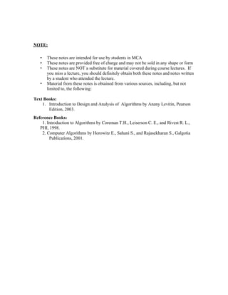
∗ Analyzing an algorithm:
There are two kinds of algorithm efficiency: time and space efficiency. Time
efficiency indicates how fast the algorithm runs; space efficiency indicates how much
extra memory the algorithm needs. Another desirable characteristic is simplicity.
Simper algorithms are easier to understand and program, the resulting programs will be
easier to debug. For e.g. Euclid’s algorithm to fid gcd (m,n) is simple than the algorithm
which uses the prime factorization. Another desirable characteristic is generality. Two
issues here are generality of the problem the algorithm solves and the range of inputs it
accepts. The designing of algorithm in general terms is sometimes easier. For eg, the
general problem of computing the gcd of two integers and to solve the problem. But at
times designing a general algorithm is unnecessary or difficult or even impossible. For
eg, it is unnecessary to sort a list of n numbers to find its median, which is its [n/2]th
smallest element. As to the range of inputs, we should aim at a range of inputs that is
natural for the problem at hand.

∗ Coding an algorithm:
Programming the algorithm by using some programming language. Formal
verification is done for small programs. Validity is done thru testing and debugging.
Inputs should fall within a range and hence require no verification. Some compilers allow
code optimization which can speed up a program by a constant factor whereas a better
algorithm can make a difference in their running time. The analysis has to be done in
various sets of inputs.

A good algorithm is a result of repeated effort & work. The program’s stopping /
terminating condition has to be set. The optimality is an interesting issue which relies on
the complexity of the problem to be solved. Another important issue is the question of
whether or not every problem can be solved by an algorithm. And the last, is to avoid
the ambiguity which arises for a complicated algorithm.

1.3 Important problem types:
The two motivating forces for any problem is its practical importance and some
specific characteristics. The different types are:
1. Sorting
2. Searching



3. String processing
4. Graph problems
5. Combinatorial problems
6. Geometric problems
7. Numerical problems.

We use these problems to illustrate different algorithm design techniques and methods
of algorithm analysis.

1. Sorting:
Sorting problem is one which rearranges the items of a given list in ascending
order. We usually sort a list of numbers, characters, strings and records similar to
college information about their students, library information and company information is
chosen for guiding the sorting technique. For eg in student’s information, we can sort it
either based on student’s register number or by their names. Such pieces of information
is called a key. The most important when we use the searching of records. There are
different types of sorting algorithms. There are some algorithms that sort an arbitrary
of size n using nlog2n comparisons, On the other hand, no algorithm that sorts by key
comparisons can do better than that. Although some algorithms are better than others,
there is no algorithm that would be the best in all situations. Some algorithms are simple
but relatively slow while others are faster but more complex. Some are suitable only for
lists residing in the fast memory while others can be adapted for sorting large files
stored on a disk, and so on.

There are two important properties. The first is called stable, if it preserves the
relative order of any two equal elements in its input. For example, if we sort the student
list based on their GPA and if two students GPA are the same, then the elements are
stored or sorted based on its position. The second is said to be ‘in place’ if it does not
require extra memory. There are some sorting algorithms that are in place and those
that are not.

2. Searching:
The searching problem deals with finding a given value, called a search key, in a
given set. The searching can be either a straightforward algorithm or binary search
algorithm which is a different form. These algorithms play a important role in real-life
applications because they are used for storing and retrieving information from large
databases. Some algorithms work faster but require more memory, some are very fast
but applicable only to sorted arrays. Searching, mainly deals with addition and deletion



of records. In such cases, the data structures and algorithms are chosen to balance
among the required set of operations.

3.String processing:
A String is a sequence of characters. It is mainly used in string handling
algorithms. Most common ones are text strings, which consists of letters, numbers and
special characters. Bit strings consist of zeroes and ones. The most important problem
is the string matching, which is used for searching a given word in a text. For e.g.
sequential searching and brute- force string matching algorithms.

4. Graph problems:
One of the interesting area in algorithmic is graph algorithms. A graph is a
collection of points called vertices which are connected by line segments called edges.
Graphs are used for modeling a wide variety of real-life applications such as
transportation and communication networks.

It includes graph traversal, shortest-path and topological sorting algorithms.
Some graph problems are very hard, only very small instances of the problems can be
solved in realistic amount of time even with fastest computers. There are two common
problems: the traveling salesman problem, finding the shortest tour through n cities
that visits every city exactly once. The graph-coloring problem is to assign the smallest
number of colors to vertices of a graph so that no two adjacent vertices are of the
same color. It arises in event-scheduling problem, where the events are represented by
vertices that are connected by an edge if the corresponding events cannot be scheduled
in the same time, a solution to this graph gives an optimal schedule.

5.Combinatorial problems:
The traveling salesman problem and the graph-coloring problem are examples of
combinatorial problems. These are problems that ask us to find a combinatorial object
such as permutation, combination or a subset that satisfies certain constraints and has
some desired (e.g. maximizes a value or minimizes a cost).
These problems are difficult to solve for the following facts. First, the number of
combinatorial objects grows extremely fast with a problem’s size. Second, there are no
known algorithms, which are solved in acceptable amount of time.

6.Geometric problems:
Geometric algorithms deal with geometric objects such as points, lines and polygons.
It also includes various geometric shapes such as triangles, circles etc. The applications
for these algorithms are in computer graphic, robotics etc.



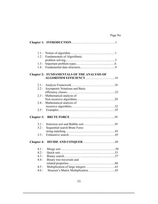
The two problems most widely used are the closest-pair problem, given ‘n’ points in
the plane, find the closest pair among them. The convex-hull problem is to find the
smallest convex polygon that would include all the points of a given set.

7.Numerical problems:
This is another large special area of applications, where the problems involve
mathematical objects of continuous nature: solving equations computing definite
integrals and evaluating functions and so on. These problems can be solved only
approximately. These require real numbers, which can be represented in a computer only
approximately. If can also lead to an accumulation of round-off errors. The algorithms
designed are mainly used in scientific and engineering applications.

1.4 Fundamental data structures:

Data structure play an important role in designing of algorithms, since it operates on
data. A data structure can be defined as a particular scheme of organizing related data
items. The data items range from elementary data types to data structures.

∗Linear Data structures:
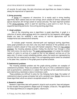
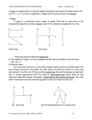
The two most important elementary data structure are the array and the linked list.
Array is a sequence contiguously in computer memory and made accessible by specifying
a value of the array’s index.

Item [0] item[1] - - - item[n-1]

Array of n elements.

The index is an integer ranges from 0 to n-1. Each and every element in the array takes
the same amount of time to access and also it takes the same amount of computer
storage.

Arrays are also used for implementing other data structures. One among is the string: a
sequence of alphabets terminated by a null character, which specifies the end of the
string. Strings composed of zeroes and ones are called binary strings or bit strings.
Operations performed on strings are: to concatenate two strings, to find the length of
the string etc.



A linked list is a sequence of zero or more elements called nodes each containing
two kinds of information: data and a link called pointers, to other nodes of the linked
list. A pointer called null is used to represent no more nodes. In a singly linked list, each
node except the last one contains a single pointer to the next element.
item 0 item 1 ………………… item n-1 null
Singly linked list of n elements.

To access a particular node, we start with the first node and traverse the pointer
chain until the particular node is reached. The time needed to access depends on where
in the list the element is located. But it doesn’t require any reservation of computer
memory, insertions and deletions can be made efficiently.

There are various forms of linked list. One is, we can start a linked list with a
special node called the header. This contains information about the linked list such as
its current length, also a pointer to the first element, a pointer to the last element.

Another form is called the doubly linked list, in which every node, except the
first and the last, contains pointers to both its success or and its predecessor.

The another more abstract data structure called a linear list or simply a list. A
list is a finite sequence of data items, i.e., a collection of data items arranged in a
certain linear order. The basic operations performed are searching for, inserting and
deleting on element.

Two special types of lists, stacks and queues. A stack is a list in which insertions
and deletions can be made only at one end. This end is called the top. The two operations
done are: adding elements to a stack (popped off). Its used in recursive algorithms,
where the last- in- first- out (LIFO) fashion is used. The last inserted will be the first
one to be removed.

A queue, is a list for, which elements are deleted from one end of the structure,
called the front (this operation is called dequeue), and new elements are added to the
other end, called the rear (this operation is called enqueue). It operates in a first- in-
first-out basis. Its having many applications including the graph problems.

A priority queue is a collection of data items from a totally ordered universe. The
principal operations are finding its largest elements, deleting its largest element and
adding a new element. A better implementation is based on a data structure called a
heap.



∗Graphs:
A graph is informally thought of a collection of points in a plane called vertices or
nodes, some of them connected by line segments called edges or arcs. Formally, a graph
G=<V, E > is defined by a pair of two sets: a finite set V of items called vertices and a
set E of pairs of these items called edges. If these pairs of vertices are unordered, i.e.
a pair of vertices (u, v) is same as (v, u) then G is undirected; otherwise, the edge (u, v),
is directed from vertex u to vertex v, the graph G is directed. Directed graphs are also
called digraphs.

Vertices are normally labeled with letters / numbers

A C B A C B

D E F D E F
1. (a) Undirected graph 1.(b) Digraph

The 1st graph has 6 vertices and seven edges.

V = {a, b, c, d, e,f },
E = {(a,c) ,( a,d ), (b,c), (b,f ), (c,e),( d,e ), (e,f) }

The digraph has four vertices and eight directed edges:

V = {a, b, c, d, e, f},
E = {(a,c), (b,c), (b,f), (c,e), (d,a), (d, e), (e,c), (e,f) }

Usually, a graph will not be considered with loops, and it disallows multiple edges
between the same vertices. The inequality for the number of edges | E | possible in an
undirected graph with |v| vertices and no loops is :

0 <= | E | < =| v | ( | V | - ) / 2.

A graph with every pair of its vertices connected by an edge is called complete.
Notation with |V| vertices is K|V| . A graph with relatively few possible edges missing is
called dense; a graph with few edges relative to the number of its vertices is called
sparse.



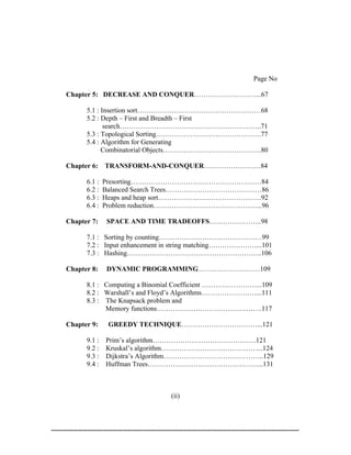
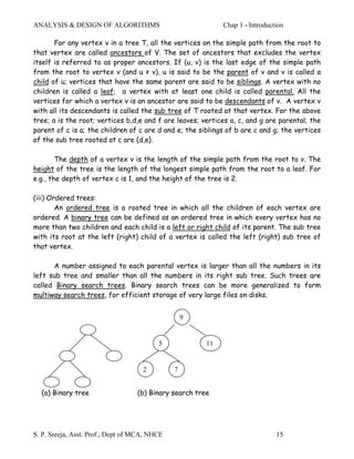
For most of the algorithm to be designed we consider the (i). Graph representation
(ii). Weighted graphs and (iii). Paths and cycles.

(i) Graph representation:

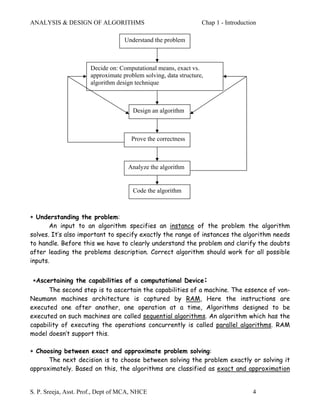
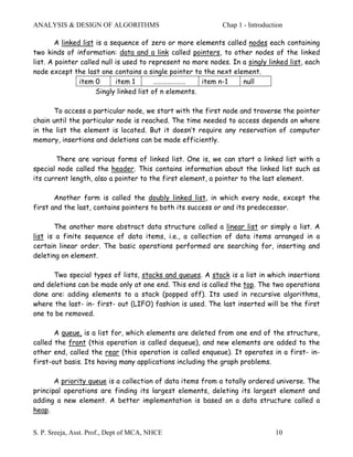
Graphs for computer algorithms can be represented in two ways: the adjacency
matrix and adjacency linked lists. The adjacency matrix of a graph with n vertices is a
n*n Boolean matrix with one row and one column for each of the graph’s vertices, in
which the element in the ith row and jth column is equal to 1 if there is an edge from the
ith vertex to the jth vertex and equal to 0 if there is no such edge.The adjacency matrix
for the undirected graph is given below:
Note: The adjacency matrix of an undirected graph is symmetric. i.e. A [i, j] = A[j, i] for
all 0 ≤ i,j ≤ n-1.

a b c d e f
a 0 0 1 1 0 0 a c d
b 0 0 1 0 0 1 b c f
c 1 1 0 0 1 0 c a b e
d 1 0 0 0 1 0 d a e
e 0 0 1 1 0 1 e c d f
f 0 1 0 0 1 0 f b e

1.(c) adjacency matrix 1.(d) adjacency linked list

The adjacency linked lists of a graph or a digraph is a collection of linked lists, one for
each vertex, that contain all the vertices adjacent to the lists vertex. The lists indicate
columns of the adjacency matrix that for a given vertex, contain 1’s. The lists consumes
less space if it’s a sparse graph.

(ii) Weighted graphs:
A weighted graph is a graph or digraph with numbers assigned to its edges. These
numbers are weights or costs. The real-life applications are traveling salesman problem,
Shortest path between two points in a transportation or communication network.

The adjacency matrix. A [i, j] will contain the weight of the edge from the ith
vertex to the jth vertex if there exist an edge; else the value will be 0 or ∞, depends on



the problem. The adjacency linked list consists of the nodes name and also the weight of
the edges.

5 a b c d
A B a ∞ 5 1 ∞ a b,5 c,1
1 7 4 b 5 ∞ 7 4 b a,5 c,7 d,4
C 1 7 ∞ 2 c a,1 b,7 d,2
C 2 D d ∞ 4 2 ∞ d b,4 c,2

2(a) weighted graph 2(b) adjacency matrix 2(c) adjacency linked list

(iii) Paths and cycles:
Two properties: Connectivity and acyclicity are important for various applications,
which depends on the notion of a path. A path from vertex v to vertex u of a graph G
can be defined as a sequence of adjacent vertices that starts with v and ends with u. If
all edges of a path are distinct, the path is said to be simple. The length of a path is the
total number of vertices in a vertex minus one. For e.g. a, c, b, f is a simple path of
length 3 from a to f and a, c, e, c, b, f is a path (not simple) of length 5 from a to f
(graph 1.a)

A directed path is a sequence of vertices in which every consecutive pair of the
vertices is connected by an edge directed from the vertex listed first to the vertex
listed next. For e.g. a, c, e, f, is a directed path from a to f in the above graph 1. (b).

A graph is said to be connected if for every pair of its vertices u and v there is a
path from u to v. If a graph is not connected, it will consist of several connected pieces
that are called connected components of the graph. A connected component is the
maximal subgraph of a given graph. The graphs (a) and (b) represents connected and not
connected graph. For e. g. in (b) there is no path from a to f. it has two connected
components with vertices {a, b, c, d, e} and {f, g, h, i}.

a c b a f

b c e g h

d e f d i
3.(a) connected graph (b) graph that is not connected.



A cycle is a simple path of a positive length that starts and end at the same vertex. For
e.g. f, h, i, g, f is a cycle in graph (b). A graph with no cycles is said to be acyclic.

∗ Trees:
A tree is a connected acyclic graph. A graph that has no cycles but is not
necessarily connected is called a forest: each of its connected components is a tree.

a b a b h

c d c d e i

f g f g j

4.(a) Trees (b) forest

Trees have several important properties :
(i) The number of edges in a tree is always one less than the number of its vertices:
|E|= |V| - 1.
(ii) Rooted trees:
For every two vertices in a tree there always exists exactly one simple path from
one of these vertices to the other. For this, select an arbitrary vertex in a free tree
and consider it as the root of the so-called rooted tree. Rooted trees plays an important
role in various applications with the help of state-space-tree which leads to two
important algorithm design techniques: backtracking and branch-and-bound. The root
starts from level 0 and the vertices adjacent to the root below is level 1 etc.

d b a

c a g b c g

e f d ef
(a) free tree (b) its transformation into a rooted tree



For any vertex v in a tree T, all the vertices on the simple path from the root to
that vertex are called ancestors of V. The set of ancestors that excludes the vertex
itself is referred to as proper ancestors. If (u, v) is the last edge of the simple path
from the root to vertex v (and u ≠ v), u is said to be the parent of v and v is called a
child of u; vertices that have the same parent are said to be siblings. A vertex with no
children is called a leaf; a vertex with at least one child is called parental. All the
vertices for which a vertex v is an ancestor are said to be descendants of v. A vertex v
with all its descendants is called the sub tree of T rooted at that vertex. For the above
tree; a is the root; vertices b,d,e and f are leaves; vertices a, c, and g are parental; the
parent of c is a; the children of c are d and e; the siblings of b are c and g; the vertices
of the sub tree rooted at c are {d,e}.

The depth of a vertex v is the length of the simple path from the root to v. The
height of the tree is the length of the longest simple path from the root to a leaf. For
e.g., the depth of vertex c is 1, and the height of the tree is 2.

(iii) Ordered trees:
An ordered tree is a rooted tree in which all the children of each vertex are
ordered. A binary tree can be defined as an ordered tree in which every vertex has no
more than two children and each child is a left or right child of its parent. The sub tree
with its root at the left (right) child of a vertex is called the left (right) sub tree of
that vertex.

A number assigned to each parental vertex is larger than all the numbers in its
left sub tree and smaller than all the numbers in its right sub tree. Such trees are
called Binary search trees. Binary search trees can be more generalized to form
multiway search trees, for efficient storage of very large files on disks.

9

5 11

2 7

(a) Binary tree (b) Binary search tree



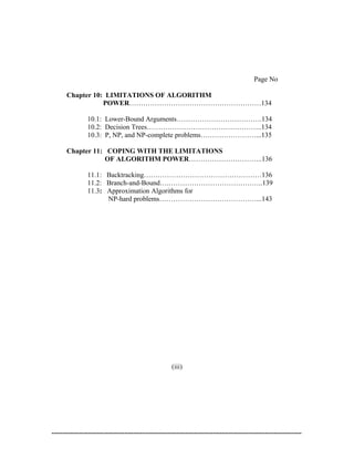
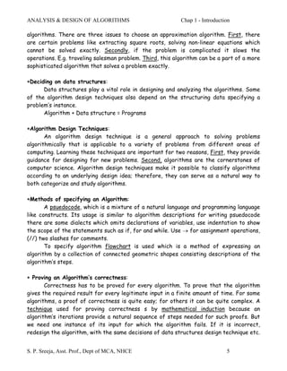
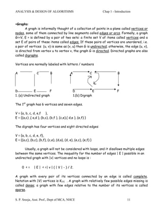
The efficiency of algorithms depends on the tree’s height for a binary search
tree. Therefore the height h of a binary tree with n nodes follows an inequality for the
efficiency of those algorithms;
[log2n] ≤ h ≤ n-1.

The binary search tree can be represented with the help of linked list: by using
just two pointers. The left pointer point to the first child and the right pointer points
to the next sibling. This representation is called the first child-next sibling
representation. Thus all the siblings of a vertex are linked in a singly linked list, with the
first element of the list pointed to by the left pointer of their parent. The ordered
tree of this representation can be rotated 45´ clock wise to form a binary tree.

9

5 null 11 null

null 2 null null 7 null
Standard implementation of binary search tree (using linked list)

a null

b d null e null

null c null f null
First-child next sibling



a

b

c d

f e

Its binary tree representation

* Sets and Dictionaries:
A set can be described as an unordered collection of distinct items called
elements of the set. A specific set is defined either by an explicit listing of its
elements or by specifying a set of property.
Sets can be implemented in computer applications in two ways. The first considers
only sets that are subsets of some large set U called the universal set. If set U has n
elements, then any subset S of U can be represented by a bit string of size n, called a
bit vector, in which the ith element is 1 iff the ith element of U is included in set S. For
e.g. if U = {1, 2, 3, 4, 5, 6, 7, 8, 9} then S = { 2, 3, 4, 7} can be represented by the bit
string as 011010100. Bit string operations are faster but consume a large amount of
storage. A multiset or bag is an unordered collection of items that are not necessarily
distinct. Note, changing the order of the set elements does not change the set, whereas
the list is just opposite. A set cannot contain identical elements, a list can.
The operation that has to be performed in a set is searching for a given item,
adding a new item, and deletion of an item from the collection. A data structure that
implements these three operations is called the dictionary. A number of applications in
computing require a dynamic partition of some n-element set into a collection of disjoint
subsets. After initialization, it performs a sequence of union and search operations. This
problem is called the set union problem.
These data structure play an important role in algorithms efficiency, which leads
to an abstract data type (ADT): a set of abstract objects representing data items with
a collection of operations that can be performed on them. Abstract data types are
commonly used in object oriented languages, such as C++ and Java, that support abstract
data types by means of classes.
*****


ANALYSIS & DESIGN OF ALGORITHMS Chap 2 Fundamentals of the Algm. efficiency

Chapter 2. Fundamentals of the Analysis of Algorithm Efficiency.

Introduction:

This chapter deals with analysis of algorithms. The American Heritage Dictionary
defines “analysis” as the “seperation of an intellectual or substantantial whole into its
constituent parts for individual study”. Algorithm’s efficiency is determined with
respect to two resources: running time and memory space. Efficiency is studied first in
quantitative terms unlike simplicity and generality. Second, give the speed and memory
of today’s computers, the efficiency consideration is of practical importance.

The algorithm’s efficiency is represented in three notations: 0 (“big oh”), Ω (“big
omega”) and θ (“big theta”). The mathematical analysis shows the framework
systematically applied to analyzing the efficiency of nonrecursive algorithms. The main
tool of such an analysis is setting up a sum representing the algorithm’s running time and
then simplifying the sum by using standard sum manipulation techniques.

2.1 Analysis Framework

For analyzing the efficiency of algorithms the two kinds are time efficiency and
space efficiency. Time efficiency indicates how fast an algorithm in question runs; space
efficiency deals with the extra space the algorithm requires. The space requirement is
not of much concern, because now we have the fast main memory, cache memory etc. so
we concentrate more on time efficiency.

• Measuring an Input’s size:

Almost all algorithms run longer on larger inputs. For example, it takes to sort
larger arrays, multiply larger matrices and so on. It is important to investigate an
algorithm’s efficiency as a function of some parameter n indicating the algorithm’s input
size. For example, it will be the size of the list for problems of sorting, searching etc.
For the problem of evaluating a polynomial p (x) = an xn+ ------+ a0 of degree n, it will be
the polynomial’s degree or the number of its coefficients, which is larger by one than its
degree.

The size also be influenced by the operations of the algorithm. For e.g., in a spell-
check algorithm, it examines individual characters of its input, then we measure the size
by the number of characters or words.

S.P. Sreeja, Asst. Prof., Dept. of MCA, NHCE 18


Note: measuring size of inputs for algorithms involving properties of numbers. For such
algorithms, computer scientists prefer measuring size by the number b of bits in the n’s
binary representation.
b= log2n+1.

• Units for measuring Running time:

We can use some standard unit of time to measure the running time of a program
implementing the algorithm. The drawbacks to such an approach are: the dependence on
the speed of a particular computer, the quality of a program implementing the algorithm.
The drawback to such an approach are : the dependence on the speed of a particular
computer, the quality of a program implementing the algorithm, the compiler used to
generate its machine code and the difficulty in clocking the actual running time of the
program. Here, we do not consider these extraneous factors for simplicity.

One possible approach is to count the number of times each of the algorithm’s
operations is executed. The simple way, is to identify the most important operation of
the algorithm, called the basic operation, the operation contributing the most to the
total running time and compute the umber of times the basic operation is executed.

The basic operation is usually the most time consuming operation in the
algorithm’s inner most loop. For example, most sorting algorithm works by comparing
elements (keys), of a list being sorted with each other; for such algorithms, the basic
operation is the key comparison.

Let Cop be the time of execution of an algorithm’s basic operation on a particular
computer and let c(n) be the number of times this operations needs to be executed for
this algorithm. Then we can estimate the running time, T (n) as:

T (n) ∼ Cop c(n)
Here, the count c(n) does not contain any information about operations that are
not basic and in tact, the count itself is often computed only approximately. The
constant Cop is also an approximation whose reliability is not easy to assess. If this
algorithm is executed in a machine which is ten times faster than one we have, the
running time is also ten times or assuming that C(n) = ½ n(n-1), how much longer will the
algorithm run if we doubt its input size? The answer is four times longer. Indeed, for
all but very small values of n,

C(n) = ½ n(n-1) = ½ n2- ½ n ≈ ½ n2



and therefore,
T(2n) Cop C(2n) ½(2n)2 = 4
T(n) ≈ Cop C(n) ≈ ½(2n)2

Here Cop is unknown, but still we got the result, the value is cancelled out in the ratio.
Also, ½ the multiplicative constant is also cancelled out. Therefore, the efficiency
analysis framework ignores multiplicative constants and concentrates on the counts’
order of growth to within a constant multiple for large size inputs.

• Orders of Growth:

This is mainly considered for large input size. On small inputs if there is
difference in running time it cannot be treated as efficient one.

Values of several functions important for analysis of algorithms:

n log2n n n log2n n2 n3 2n n!
10 3.3 101 3.3 x 101 102 10 3
10 3
3.6 x 106
102 6.6 102 6.6 x 102 104 106 1.3 x 1030 9.3 x 10157
103 10 103 1.0 x 104 106 109
104 13 104 1.3 x 105 108 1012
105 17 105 1.7 x 106 1010 1015
106 20 106 2.0 x 107 1012 1018

The function growing slowly is the logarithmic function, logarithmic basic-
operation count to run practically instantaneously on inputs of all realistic sizes.
Although specific values of such a count depend, of course, in the logarithm’s base, the
formula

logan = logab x logbn

Makes it possible to switch from one base to another, leaving the count logarithmic but
with a new multiplicative constant.

On the other end, the exponential function 2n and the factorial function n! grow
so fast even for small values of n. These two functions are required to as exponential-
growth functions. “Algorithms that require an exponential number of operations are
practical for solving only problems of very small sizes.”



Another way to appreciate the qualitative difference among the orders of growth
of the functions is to consider how they react to, say, a twofold increase in the value of
their argument n. The function log2n increases in value by just 1 (since log22n = log22 +
log2n = 1 + log2n); the linear function increases twofold; the nlogn increases slightly
more than two fold; the quadratic n2 as fourfold ( since (2n)2 = 4n2) and the cubic
function n3 as eight fold (since (2n)3 = 8n3); the value of 2n is squared (since 22n = (2n)2
and n! increases much more than that.

• Worst-case, Best-case and Average-case efficiencies:

The running time not only depends on the input size but also on the specifics of a
particular input. Consider the example, sequential search. It’s a straightforward
algorithm that searches for a given item (search key K) in a list of n elements by
checking successive elements of the list until either a match with the search key is
found or the list is exhausted.

The psuedocode is as follows.

Algorithm sequential search {A [0. . n-1] , k }
// Searches for a given value in a given array by Sequential search
// Input: An array A[0..n-1] and a search key K
// Output: Returns the index of the first element of A that matches K or -1 if there is
// no match
i← o
while i< n and A [ i ] ≠ K do
i← i+1
if i< n return i
else return –1

Clearly, the running time of this algorithm can be quite different for the same
list size n. In the worst case, when there are no matching elements or the first
matching element happens to be the last one on the list, the algorithm makes the largest
number of key comparisons among all possible inputs of size n; Cworst (n) = n.

The worst-case efficiency of an algorithm is its efficiency for the worst-case
input of size n, which is an input of size n for which the algorithm runs the longest
among all possible inputs of that size. The way to determine is, to analyze the algorithm
to see what kind of inputs yield the largest value of the basic operation’s count c(n)
among all possible inputs of size n and then compute this worst-case value Cworst (n).



The best-case efficiency of an algorithm is its efficiency for the best-case input
of size n, which is an input of size n for which the algorithm runs the fastest among all
inputs of that size. First, determine the kind of inputs for which the count C(n) will be
the smallest among all possible inputs of size n. Then ascertain the value of C(n) on the
most convenient inputs. For e.g., for the searching with input size n, if the first element
equals to a search key, Cbest(n) = 1.

Neither the best-case nor the worst-case gives the necessary information about
an algorithm’s behaviour on a typical or random input. This is the information that the
average-case efficiency seeks to provide. To analyze the algorithm’s average-case
efficiency, we must make some assumptions about possible inputs of size n.

Let us consider again sequential search. The standard assumptions are that:

(a) the probability of a successful search is equal to p (0 ≤ p ≤ 1), and,
(b) the probability of the first match occurring in the ith position is same for every i.

Accordingly, the probability of the first match occurring in the ith position of the list
is p/n for every i, and the no of comparisons is i for a successful search. In case of
unsuccessful search, the number of comparisons is n with probability of such a search
being (1-p). Therefore,

Cavg(n) = [1 . p/n + 2 . p/n + ………. i . p/n + ……….. n . p/n] + n.(1-p)

= p/n [ 1+2+…….i+……..+n] + n.(1-p)

= p/n . [n(n+1)]/2 + n.(1-p) [sum of 1st n natural number formula]

= [p(n+1)]/2 + n.(1-p)

This general formula yields the answers. For e.g, if p=1 (ie., successful), the
average number of key comparisons made by sequential search is (n+1)/2; ie, the
algorithm will inspect, on an average, about half of the list’s elements. If p=0 (ie.,
unsuccessful), the average number of key comparisons will be ‘n’ because the algorithm
will inspect all n elements on all such inputs.

The average-case is better than the worst-case, and it is not the average of both best
and worst-cases.



Another type of efficiency is called amortized efficiency. It applies not to a
single run of an algorithm but rather to a sequence of operations performed on the same
data structure. In some situations a single operation can be expensive, but the total
time for an entire sequence of such n operations is always better than the worst-case
efficiency of that single operation multiplied by n. It is considered in algorithms for
finding unions of disjoint sets.

Recaps of Analysis framework:
1) Both time and space efficiencies are measured as functions of the algorithm’s i/p
size.
2) Time efficiency is measured by counting the number of times the algorithm’s
basic operation is executed. Space efficiency is measured by counting the number
of extra memory units consumed by the algorithm.
3) The efficiencies of some algorithms may differ significantly for input of the
same size. For such algorithms, we need to distinguish between the worst-case,
average-case and best-case efficiencies.
4) The framework’s primary interest lies in the order of growth of the algorithm’s
running tine as its input size goes to infinity.

2.2 Asymptotic Notations and Basic Efficiency classes:

The efficiency analysis framework concentrates on the order of growth of an
algorithm’s basic operation count as the principal indicator of the algorithm’s efficiency.
To compare and rank such orders of growth, we use three notations; 0 (big oh), Ω (big
omega) and θ (big theta). First, we see the informal definitions, in which t(n) and g(n)
can be any non negative functions defined on the set of natural numbers. t(n) is the
running time of the basic operation, c(n) and g(n) is some function to compare the count
with.

Informal Introduction:

O [g(n)] is the set of all functions with a smaller or same order of growth as g(n)

Eg: n ∈ O (n2), 100n+5 ∈ O(n2), 1/2n(n-1) ∈ O(n2).

The first two are linear and have a smaller order of growth than g(n)=n2, while the last
one is quadratic and hence has the same order of growth as n2. on the other hand,



n3∈ (n2), 0.00001 n3 ∉ O(n2), n4+n+1 ∉ O(n 2 ).The function n3 and 0.00001 n3 are both
cubic and have a higher order of growth than n2 , and so has the fourth-degree
polynomial n4 +n+1

The second-notation, Ω [g(n)] stands for the set of all functions with a larger or
same order of growth as g(n). for eg, n3 ∈ Ω(n2), 1/2n(n-1) ∈ Ω(n2), 100n+5 ∉ Ω(n2)

Finally, θ [g(n)] is the set of all functions that have the same order of growth as g(n).

E.g, an2+bn+c with a>0 is in θ(n2)

• O-notation:

Definition: A function t(n) is said to be in 0[g(n)]. Denoted t(n) ∈ 0[g(n)], if t(n) is
bounded above by some constant multiple of g(n) for all large n ie.., there exist some
positive constant c and some non negative integer no such that t(n) ≤ cg(n) for all n≥no.

Eg. 100n+5 ∈ 0 (n2)

Proof: 100n+ 5 ≤ 100n+n (for all n ≥ 5) = 101n ≤ 101 n2
Thus, as values of the constants c and n0 required by the definition, we con take 101 and
5 respectively. The definition says that the c and n0 can be any value. For eg we can also
take. C = 105,and n0 = 1.

i.e., 100n+ 5 ≤ 100n + 5n (for all n ≥ 1) = 105n

cg(n)

f t(n)

n0 n



• Ω-Notation:

Definition: A fn t(n) is said to be in Ω[g(n)], denoted t(n) ∈Ω[g(n)], if t(n) is bounded
below by some positive constant multiple of g(n) for all large n, ie., there exist some
positive constant c and some non negative integer n0 s.t.
t(n) ≥ cg(n) for all n ≥ n0.

For example: n3 ∈ Ω(n2), Proof is n3 ≥ n2 for all n ≥ n0. i.e., we can select c=1 and n0=0.

t(n)

f cg(n)

n0 n

• θ - Notation:

Definition: A function t(n) is said to be in θ [g(n)], denoted t(n)∈ θ (g(n)), if t(n) is
bounded both above and below by some positive constant multiples of g(n) for all large n,
ie., if there exist some positive constant c1 and c2 and some nonnegative integer n0 such
that c2g(n) ≤ t(n) ≤ c1g(n) for all n ≥ n0.

Example: Let us prove that ½ n(n-1) ∈ θ( n2 ) .First, we prove the right inequality (the
upper bound)
½ n(n-1) = ½ n2 – ½ n ≤ ½ n2 for all n ≥ n0.
Second, we prove the left inequality (the lower bound)
½ n(n-1) = ½ n2 – ½ n ≥ ½ n2 – ½ n½ n for all n ≥ 2 = ¼ n2.
Hence, we can select c2= ¼, c2= ½ and n0 = 2



c1g(n)

f tg(n)
c2g(n)

n0 n

Useful property involving these Notations:

The property is used in analyzing algorithms that consists of two consecutively executed
parts:

THEOREM If t1(n) Є O(g1(n)) and t2(n) Є O(g2(n)) then t1 (n) + t2(n) Є O(max{g1(n),
g2(n)}).
PROOF (As we shall see, the proof will extend to orders of growth the following simple
fact about four arbitrary real numbers a1 , b1 , a2, and b2: if a1 < b1 and a2 < b2 then a1 + a2 < 2 max{
b1, b2}.) Since t1(n) Є O(g1(n)) , there exist some constant c and some nonnegative integer n 1
such that
t1(n) < c1g1 (n) for all n > n1
since t2(n) Є O(g2(n)),
t2(n) < c2g2(n) for all n > n2.

Let us denote c3 = maxfc1, c2} and consider n > max{ n1 , n2} so that we can use both
inequalities. Adding the two inequalities above yields the following:
t1(n) + t2(n) < c1g1 (n) + c2g2(n)
< c3g1(n) + c3g2(n) = c3 [g1(n) + g2(n)]
< c32max{g1 (n),g2(n)}.

Hence, t1 (n) + t2(n) Є O(max {g1(n) , g2(n)}), with the constants c and n0 required by
the O definition being 2c3 = 2 max{c1, c2} and max{n1, n 2 }, respectively.



This implies that the algorithm's overall efficiency will be determined by the part with
a larger order of growth, i.e., its least efficient part:
t1(n) Є O(g1(n))
t2(n) Є O(g2(n)) then t1 (n) + t2(n) Є O(max{g1(n), g2(n)}).

For example, we can check whether an array has identical elements by means of the
following two-part algorithm: first, sort the array by applying some known sorting algorithm;
second, scan the sorted array to check its consecutive elements for equality. If, for example,
a sorting algorithm used in the first part makes no more than 1/2n(n — 1) comparisons (and
hence is in O(n2)) while the second part makes no more than n — 1 comparisons (and hence is
in O(n}), the efficiency of the entire algorithm will be in
(O(max{n2, n}) = O(n2).

Using Limits for Comparing Orders of Growth:

The convenient method for doing the comparison is based on computing the limit of
the ratio of two functions in question. Three principal cases may arise:
t(n) 0 implies that t(n) has a smaller order of growth than g(n)
lim —— = c implies that t ( n ) has the same order of growth as g(n)

n ->
∞ g(n) ∞ implies that t (n) has a larger order of growth than g(n).
Note that the first two cases mean that t ( n ) Є O(g(n)), the last two mean that
t(n) Є Ω(g(n)), and the second case means that t(n) Є θ(g(n)).

EXAMPLE 1 Compare orders of growth of ½ n(n - 1) and n2. (This is one of the
examples we did above to illustrate the definitions.)
lim ½ n(n-1) = ½ lim n2 – n = ½ lim (1- 1/n ) = ½
n ->∞ n2 n ->∞ n2 n ->∞

Since the limit is equal to a positive constant, the functions have the same order of
growth or, symbolically, ½ n(n - 1) Є θ (n2)

Basic Efficiency Classes :
Even though the efficiency analysis framework puts together all the functions
whose orders of growth differ by a constant multiple, there are still infinitely many such
classes. (For example, the exponential functions an have different orders of growth for
different values of base a.) Therefore, it may come as a surprise that the time efficiencies



of a large number of algorithms fall into only a few classes. These classes are listed in Table
in increasing order of their orders of growth, along with their names and a few comments.

You could raise a concern that classifying algorithms according to their asymptotic
efficiency classes has little practical value because the values of multiplicative constants are
usually left unspecified. This leaves open a possibility of an algorithm in a worse efficiency class
running faster than an algorithm in a better efficiency class for inputs of realistic sizes. For
example, if the running time of one algorithm is n3 while the running time of the other is
106n2, the cubic algorithm will outperform the quadratic algorithm unless n exceeds 106. A
few such anomalies are indeed known. For example, there exist algorithms for matrix
multiplication with a better asymptotic efficiency than the cubic efficiency of the definition-
based algorithm (see Section 4.5). Because of their much larger multiplicative constants,
however, the value of these more sophisticated algorithms is mostly theoretical.

Fortunately, multiplicative constants usually do not differ that drastically. As a rule,
you should expect an algorithm from a better asymptotic efficiency class to outperform an
algorithm from a worse class even for moderately sized inputs. This observation is especially
true for an algorithm with a better than exponential running time versus an exponential (or
worse) algorithm.

Class Name Comments
1 Constant Short of best case efficiency when its input grows
the time also grows to infinity.
logn Logarithmic It cannot take into account all its input, any algorithm
that does so will have atleast linear running time.
n Linear Algorithms that scan a list of size n, eg., sequential
search
nlogn nlogn Many divide & conquer algorithms including
mergersort quicksort fall into this class
n2 Quadratic Characterizes with two embedded loops, mostly
sorting and matrix operations.
n3 Cubic Efficiency of algorithms with three embedded loops,
2n Exponential Algorithms that generate all subsets of an n-element
set
n! factorial Algorithms that generate all permutations of an n-
element set



2.3 Mathematical Analysis of Non recursive
Algorithms:
In this section, we systematically apply the general framework outlined in Section 2.1
to analyzing the efficiency of nonrecursive algorithms. Let us start with a very simple
example that demonstrates all the principal steps typically taken in analyzing such algorithms.
EXAMPLE 1 Consider the problem of finding the value of the largest element in a list
of n numbers. For simplicity, we assume that the list is implemented as an array. The
following is a pseudocode of a standard algorithm for solving the problem.
ALGORITHM MaxElement(A[0,..n - 1])
//Determines the value of the largest element in a given array
//Input: An array A[0..n - 1] of real numbers
//Output: The value of the largest element in A
maxval <- A[0]
for i <- 1 to n - 1 do
if A[i] > maxval
maxval <— A[i]
return maxval
The obvious measure of an input's size here is the number of elements in the array,
i.e., n. The operations that are going to be executed most often are in the algorithm's for
loop. There are two operations in the loop's body: the comparison A[i] > maxval and the
assignment maxval <- A[i]. Since the comparison is executed on each repetition of the loop
and the assignment is not, we should consider the comparison to be the algorithm's basic
operation. (Note that the number of comparisons will be the same for all arrays of size n;
therefore, in terms of this metric, there is no need to distinguish among the worst, average,
and best cases here.)

Let us denote C(n) the number of times this comparison is executed and try to find a
formula expressing it as a function of size n. The algorithm makes one comparison on each
execution of the loop, which is repeated for each value of the loop's variable i within the
bounds between 1 and n — 1 (inclusively). Therefore, we get the following sum for C(n):

n-1
C(n) = ∑ 1
i=1

This is an easy sum to compute because it is nothing else but 1 repeated n — 1 times.
Thus,



n-1
C(n) = ∑ 1 = n-1 Є θ(n)
i=1
Here is a general plan to follow in analyzing nonrecursive algorithms.

General Plan for Analyzing Efficiency of Nonrecursive Algorithms
1. Decide on a parameter (or parameters) indicating an input's size.
2. Identify the algorithm's basic operation. (As a rule, it is located in its innermost
loop.)
3. Check whether the number of times the basic operation is executed depends only
on the size of an input. If it also depends on some additional property, the worst-
case, average-case, and, if necessary, best-case efficiencies have to be
investigated separately.
4. Set up a sum expressing the number of times the algorithm's basic operation is
executed.
5. Using standard formulas and rules of sum manipulation either find a closed-form
formula for the count or, at the very least, establish its order of growth.

In particular, we use especially frequently two basic rules of sum manipulation
u u
∑ c ai = c ∑ ai ----(R1)
i=1 i=1

u u u
∑ (ai ± bi) = ∑ ai ± ∑ bi ----(R2)
i=1 i=1 i=1
and two summation formulas
u
∑ 1 = u- l + 1 where l ≤ u are some lower and upper integer limits --- (S1 )
i=l
n
∑ i = 1+2+….+n = [n(n+1)]/2 ≈ ½ n2 Є θ(n2) ----(S2)
i=0

(Note that the formula which we used in Example 1, is a special case of formula (S1)
for l= = 0 and n = n - 1)



EXAMPLE 2 Consider the element uniqueness problem: check whether all the
elements in a given array are distinct. This problem can be solved by the following
straightforward algorithm.
ALGORITHM UniqueElements(A[0..n - 1])
//Checks whether all the elements in a given array are distinct
//Input: An array A[0..n - 1]
//Output: Returns "true" if all the elements in A are distinct
// and "false" otherwise.
for i «— 0 to n — 2 do
for j' <- i: + 1 to n - 1 do
if A[i] = A[j]
return false
return true
The natural input's size measure here is again the number of elements in the
array, i.e., n. Since the innermost loop contains a single operation (the comparison of two
elements), we should consider it as the algorithm's basic operation. Note, however, that
the number of element comparisons will depend not only on n but also on whether there are
equal elements in the array and, if there are, which array positions they occupy. We will limit
our investigation to the worst case only.

By definition, the worst case input is an array for which the number of element
comparisons Cworst(n) is the largest among all arrays of size n. An inspection of the innermost
loop reveals that there ate two kinds of worst-case inputs (inputs for which the algorithm
does not exit the loop prematurely): arrays with no equal elements and arrays in which the
last two elements are the only pair of equal elements. For such inputs, one comparison is
made for each repetition of the innermost loop, i.e., for each value of the loop's variable j
between its limits i + 1 and n - 1; and this is repeated for each value of the outer loop, i.e., for
each value of the loop's variable i between its limits 0 and n - 2. Accordingly, we get

n-2 n-1 n-2 n-2
C worst (n) = ∑ ∑ 1 = ∑ [(n-1) – (i+1) + 1] = ∑ (n-1-i)
i=0 j=i+1 i=0 i=0

n-2 n-2 n-2
= ∑ (n-1) - ∑ i = (n-1) ∑ 1 – [(n-2)(n-1)]/2
i=0 i=0 i=0

= (n-1) 2 - [(n-2)(n-1)]/2 = [(n-1)n]/2 ≈ ½ n2 Є θ(n2)
Also it can be solved as (by using S2)



n-2
∑ (n-1-i) = (n-1) + (n-2) + ……+ 1 = [(n-1)n]/2 ≈ ½ n2 Є θ(n2)
i=0
Note that this result was perfectly predictable: in the worst case, the algorithm
needs to compare all n(n - 1)/2 distinct pairs of its n elements.

2.4 Mathematical Analysis of Recursive Algorithms:

In this section, we systematically apply the general framework to analyze the
efficiency of recursive algorithms. Let us start with a very simple example that
demonstrates all the principal steps typically taken in analyzing recursive algorithms.

Example 1: Compute the factorial function F(n) = n! for an arbitrary non negative integer
n. Since,
n! = 1 * 2 * ……. * (n-1) *n = n(n-1)! For n ≥ 1
and 0! = 1 by definition, we can compute F(n) = F(n-1).n with the following recursive
algorithm.

ALGORITHM F(n)
// Computes n! recursively
// Input: A nonnegative integer n
// Output: The value of n!
ifn =0 return 1
else return F(n — 1) * n
For simplicity, we consider n itself as an indicator of this algorithm's input size (rather
than the number of bits in its binary expansion). The basic operation of the algorithm is
multiplication, whose number of executions we denote M(n). Since the function F(n) is
computed according to the formula
F(n) = F ( n - 1 ) - n for n > 0,
the number of multiplications M(n) needed to compute it must satisfy the equality
M(n) = M(n - 1) + 1 for n > 0.
to compute to multiply
F(n-1) F(n-1) by n
Indeed, M(n - 1) multiplications are spent to compute F(n - 1), and one more
multiplication is needed to multiply the result by n.
The last equation defines the sequence M(n) that we need to find. Note that the
equation defines M(n) not explicitly, i.e., as a function of n, but implicitly as a function of its
value at another point, namely n — 1. Such equations are called recurrence relations or, for



brevity, recurrences. Recurrence relations play an important role not only in analysis of
algorithms but also in some areas of applied mathematics. Our goal now is to solve the
recurrence relation M(n) = M(n — 1) + 1, i.e., to find an explicit formula for the sequence M(n)
in terms of n only.
Note, however, that there is not one but infinitely many sequences that satisfy this
recurrence. To determine a solution uniquely, we need an initial condition that tells us the
value with which the sequence starts. We can obtain this value by inspecting the condition
that makes the algorithm stop its recursive calls:
if n = 0 return 1.
This tells us two things. First, since the calls stop when n = 0, the smallest value of n
for which this algorithm is executed and hence M(n) defined is 0. Second,by inspecting the
code's exiting line, we can see that when n = 0, the algorithm performs no multiplications.
Thus, the initial condition we are after is
M (0) = 0.
the calls stop when n = 0 ———' '—— no multiplications when n = 0
Thus, we succeed in setting up the recurrence relation and initial condition for
the algorithm's number of multiplications M(n):
M(n) = M(n - 1) + 1 for n > 0, (2.1)
M (0) = 0.
Before we embark on a discussion of how to solve this recurrence, let us pause to
reiterate an important point. We are dealing here with two recursively defined
functions. The first is the factorial function F(n) itself; it is defined by the recurrence
F(n) = F(n - 1) • n for every n > 0, F(0) = l.

The second is the number of multiplications M(n) needed to compute F(n) by the
recursive algorithm whose pseudocode was given at the beginning of the section. As we
just showed, M(n) is defined by recurrence (2.1). And it is recurrence (2.1) that we need
to solve now.

Though it is not difficult to "guess" the solution, it will be more useful to arrive
at it in a systematic fashion. Among several techniques available for solving recurrence
relations, we use what can be called the method of backward substitutions. The
method's idea (and the reason for the name) is immediately clear from the way it
applies to solving our particular recurrence:
M(n) = M(n - 1) + 1 substitute M(n - 1) = M(n - 2) + 1
= [M(n - 2) + 1] + 1 = M(n - 2) + 2 substitute M(n - 2) = M(n - 3) + 1
= [M(n - 3) + 1] + 2 = M (n - 3) + 3.
After inspecting the first three lines, we see an emerging pattern, which makes it
possible to predict not only the next line (what would it be?) but also a general formula



for the pattern: M(n) = M(n — i) + i. Strictly speaking, the correctness of this formula
should be proved by mathematical induction, but it is easier to get the solution as
follows and then verify its correctness.
What remains to be done is to take advantage of the initial condition given. Since
it is specified for n = 0, we have to substitute i = n in the pattern's formula to get the
ultimate result of our backward substitutions:
M(n) = M(n - 1) + 1 = • • • = M(n - i) + i = - ---- = M(n -n) + n = n.

The benefits of the method illustrated in this simple example will become clear very
soon, when we have to solve more difficult recurrences. Also note that the simple iterative
algorithm that accumulates the product of n consecutive integers requires the same
number of multiplications, and it does so without the overhead of time and space used for
maintaining the recursion's stack.

The issue of time efficiency is actually not that important for the problem of
computing n!, however. The function's values get so large so fast that we can realistically
compute its values only for very small n's. Again, we use this example just as a simple and
convenient vehicle to introduce the standard approach to analyzing recursive algorithms.
•
Generalizing our experience with investigating the recursive algorithm for computing
n!, we can now outline a general plan for investigating recursive algorithms.

A General Plan for Analyzing Efficiency of Recursive Algorithms
1. Decide on a parameter (or parameters) indicating an input's size.
2. Identify the algorithm's basic operation.
3. Check whether the number of times the basic operation is executed can vary on
different inputs of the same size; if it can, the worst-case, average-case, and best-
case efficiencies must be investigated separately.
4. Set up a recurrence relation, with an appropriate initial condition, for the
number of times the basic operation is executed.
5. Solve the recurrence or at least ascertain the order of growth of its solution.

Example 2: the algorithm to find the number of binary digits in the binary representation of a
positive decimal integer.
ALGORITHM BinRec(n) : -
//Input: A positive decimal integer n
//Output: The number of binary digits in n's binary representation
if n = 1 return 1
else return BinRec(n/2) + 1



Let us set up a recurrence and an initial condition for the number of additions A(n) made by
the algorithm. The number of additions made in computing BinRec(n/2) is A(n/2), plus one
more addition is made by the algorithm to increase the returned value by 1. This leads to the
recurrence
A(n) = A(n/2) + 1 for n > 1. (2.2)
Since the recursive calls end when n is equal to 1 and there are no additions made then, the
initial condition is
A(1) = 0

The presence of [n/2] in the function's argument makes the method of backward
substitutions stumble on values of n that are not powers of 2. Therefore, the standard
approach to solving such a recurrence is to solve it only for n — 2k and then take advantage
of the theorem called the smoothness rule which claims that under very broad assumptions
the order of growth observed for n = 2k gives a correct answer about the order of growth for
all values of n. (Alternatively, after getting a solution for powers of 2, we can sometimes
finetune this solution to get a formula valid for an arbitrary n.) So let us apply this recipe to
our recurrence, which for n = 2k takes the form
A(2 k) = A(2 k -1 ) + 1 for k > 0, A(2 0 ) = 0
Now backward substitutions encounter no problems:

A(2 k) = A(2 k -1 ) + 1 substitute A(2k-1) = A(2k -2) + 1
= [A(2k -2 ) + 1] + 1 = A(2k -2) + 2 substitute A(2k -2) = A(2k-3) + 1
= [A(2 k -3) + 1] + 2 = A(2 k -3) + 3
……………

= A(2 k -i) + i
……………
= A(2 k -k) + k

Thus, we end up with
A(2k) = A ( 1 ) + k = k
or, after returning to the original variable n = 2k and, hence, k = log2 n,
A ( n ) = log2 n Є θ (log n).

2.5 Example: Fibonacci numbers

In this section, we consider the Fibonacci numbers, a sequence of
numbers as 0, 1, 1, 2, 3, 5, 8, …. That can be defined by the simple recurrence



F(n) = F(n -1) + F(n-2) for n > 1 ----(2.3)
and two initial conditions
F(0) = 0, F(1) = 1 ----(2.4)
The Fibonacci numbers were introduced by Leonardo Fibonacci in 1202 as a solution to
a problem about the size of a rabbit population. Many more examples of Fibonacci-like
numbers have since been discovered in the natural world, and they have even been used in
predicting prices of stocks and commodities. There are some interesting applications of the
Fibonacci numbers in computer science as well. For example, worst-case inputs for Euclid's
algorithm happen to be consecutive elements of the Fibonacci sequence. Our discussion goals
are quite limited here, however. First, we find an explicit formula for the nth Fibonacci
number F(n), and then we briefly discuss algorithms for computing it.

Explicit Formula for the nth Fibonacci Number
If we try to apply the method of backward substitutions to solve recurrence (2.6),
we will fail to get an easily discernible pattern. Instead, let us take advantage of a
theorem that describes solutions to a homogeneous second-order linear recurrence
with constant coefficients
ax(n) + bx(n - 1) + cx(n - 2) = 0, -----(2.5)
where a, b, and c are some fixed real numbers (a ≠ 0) called the coefficients of the
recurrence and x(n) is an unknown sequence to be found. According to this theorem—see
Theorem 1 in Appendix B—recurrence (2.5) has an infinite number of solutions that can be
obtained by one of the three formulas. Which of the three formulas applies for a particular
case depends on the number of real roots of the quadratic equation with the same
coefficients as recurrence (2.5):
ar2 + br + c = 0. (2.6)
Quite logically, equation (2.6) is called the characteristic equation for recurrence (2.5).
Let us apply this theorem to the case of the Fibonacci numbers.
F(n) - F(n - 1) - F(n - 2) = 0. (2.7)
Its characteristic equation is
r 2 - r - 1 = 0,
with the roots
r 1,2 = (1 ± √1-4(-1)) /2 = (1 ± √5)/2

Algorithms for Computing Fibonacci Numbers
Though the Fibonacci numbers have many fascinating properties, we limit our
discussion to a few remarks about algorithms for computing them. Actually, the sequence
grows so fast that it is the size of the numbers rather than a time-efficient method for
computing them that should be of primary concern here. Also, for the sake of simplicity,
we consider such operations as additions and multiplications at unit cost in the algorithms



that follow. Since the Fibonacci numbers grow infinitely large (and grow rapidly), a more
detailed analysis than the one offered here is warranted. These caveats
notwithstanding, the algorithms we outline and their analysis are useful examples for a
student of design and analysis of algorithms.

To begin with, we can use recurrence (2.3) and initial condition (2.4) for the
obvious recursive algorithm for computing F(n).
ALGORITHM F(n)
//Computes the nth Fibonacci number recursively by using its definition
//Input: A nonnegative integer n
//Output: The nth Fibonacci number
if n < 1 return n
else return F(n - 1) + F(n - 2)

Analysis:
The algorithm's basic operation is clearly addition, so let A(n) be the number of
additions performed by the algorithm in computing F(n). Then the numbers of
additions needed for computing F(n — 1) and F(n — 2) are A(n — 1) and A(n — 2),
respectively, and the algorithm needs one more addition to compute their sum. Thus,
we get the following recurrence for A(n):
A(n) = A(n - 1) + A(n - 2) + 1 for n > 1, (2.8)
A(0)=0, A(1) = 0.
The recurrence A(n) — A(n — 1) — A(n — 2) = 1 is quite similar to recurrence (2.7) but
its right-hand side is not equal to zero. Such recurrences are called inhomo-geneous
recurrences. There are general techniques for solving inhomogeneous recurrences (see
Appendix B or any textbook on discrete mathematics), but for this particular
recurrence, a special trick leads to a faster solution. We can reduce our inhomogeneous
recurrence to a homogeneous one by rewriting it as
[A(n) + 1] - [A(n -1) + 1]- [A(n - 2) + 1] = 0 and substituting B(n) = A(n) + 1:
B(n) - B(n - 1) - B(n - 2) = 0
B(0) = 1, B(1) = 1.

This homogeneous recurrence can be solved exactly in the same manner as recurrence
(2.7) was solved to find an explicit formula for F(n).

We can obtain a much faster algorithm by simply computing the successive elements
of the Fibonacci sequence iteratively, as is done in the following algorithm.
ALGORITHM Fib(n)
//Computes the nth Fibonacci number iteratively by using its definition



//Input: A nonnegative integer n
//Output: The nth Fibonacci number
F[0]<-0; F[1]<-1
for i <- 2 to n do
F[i]«-F[i-1]+F[i-2]
return F[n]

This algorithm clearly makes n - 1 additions. Hence, it is linear as a function of n and
"only" exponential as a function of the number of bits b in n's binary representation.
Note that using an extra array for storing all the preceding elements of the Fibonacci
sequence can be avoided: storing just two values is necessary to accomplish the task.

The third alternative for computing the nth Fibonacci number lies in using a formula.
The efficiency of the algorithm will obviously be determined by the efficiency of an
exponentiation algorithm used for computing ø n. If it is done by simply multiplying ø by itself n
- 1 times, the algorithm will be in θ (n) = θ (2b) . There are faster algorithms for the
exponentiation problem. Note also that special care should be exercised in implementing
this approach to computing the nth Fibonacci number. Since all its intermediate results
are irrational numbers, we would have to make sure that their approximations in the
computer are accurate enough so that the final round-off yields a correct result.
Finally, there exists a θ (logn) algorithm for computing the nth Fibonacci number
that manipulates only integers. It is based on the equality
n
F(n-1) F(n) = 0 1
F(n) F(n+1) 1 1 for n ≥ 1

and an efficient way of computing matrix powers.

*****


ANALYSIS & DESIGN OF ALGORITHMS Chap 3 – Brute Force

Chapter 3. Brute Force

Introduction:

Brute force is a straightforward approach to solving a problem, usually directly
based on the problem’s statement and definitions of the concepts involved. For e.g. the
algorithm to find the gcd of two numbers.

Brute force approach is not an important algorithm design strategy for the
following reasons:

• First, unlike some of the other strategies, brute force is applicable to a very
wide variety of problems. Its used for many elementary but algorithmic
tasks such as computing the sum of n numbers, finding the largest element in
a list and so on.

• Second, for some problem it yields reasonable algorithms of at least some
practical value with no limitation on instance size.

• Third, the expense of designing a more efficient algorithm if few instances
to be solved and with acceptable speed for solving it.

• Fourth, even though it is inefficient, it can be used to solve small-instances
of a problem.

• Last, it can serve as an important theoretical or educational propose.

3.1 Selection sort and Bubble sort:

The application of Brute-force for the problem of sorting: given a list of n
orderable items(eg., numbers characters, strings etc.) , rearrange them in increasing
order. The straightforward sorting is based on two algorithms selection and bubble
sort. Selection sort is better than the bubble sorting, but, both are better algorithms
because of its clarity.

S. P. Sreeja, Asst.Prof., Dept. of MCA, NHCE 39


Selection sort:

By scanning the entire list to find its smallest element and exchange it with the
first element, putting the smallest element in its final position in the sorted list. Then
scan the list with the second element, to find the smallest among the last n-1 elements
and exchange it with second element. Continue this process till the n-2 elements.
Generally, in the ith pass through the list, numbered 0 to n-2, the algorithm searches
for the smallest item among the last n-i elements and swaps it with Ai.

A0 ≤ A1 ≤ ……….. ≤ Ai-1 Ai, ………… Amin , ………. An-1
in their final positions the last n-i elements
After n-1 passes the list is sorted

Algorithm selection sort (A[0…n-1])
// The algorithm sorts a given array
//Input: An array A[0..n-1] of orderable elements
// Output: Array A[0..n-1] sorted increasing order
for i← 0 to n-2 do
min ← i
for j← i + 1 to n-1 do
if A[j] < A[min] min← j
swap A[i] and A[min]

The e.g. for the list 89,45,68,90,29,34,17 is

89 45 68 90 29 34 17
17

17 45 68 90 29
29 34 89

17 29 68 90 45 34
34 89

17 29 34 90 45 68 89

17 29 34 45 90 68 89

17 29 34 45 68 90 89

17 29 34 45 68 89 90



Analysis:

The input’s size is the no of elements ‘n’’ the algorithms basic operation is the key
comparison A[j]<A[min]. The number of times it is executed depends on the array size
and it is the summation:
n-2 n-1
C(n) = ∑ ∑ 1
i=0 j=i+1

n-2
= ∑ [ (n-1) – (i+1) + 1]
i=0
n-2
=∑ ( n-1-i)
i=0

Either compute this sum by distributing the summation symbol or by immediately getting
the sum of decreasing integers:, it is

n-2 n-1
C(n) = ∑ ∑ 1
i=0 j=i+1

n-2
= ∑ (n-1 - i)
i=0
= [n(n-1)]/2

Thus selection sort is a θ(n2) algorithm on all inputs. Note, The number of key swaps is
only θ(n), or n-1.

Bubble sort:

It is based on the comparisons of adjacent elements and exchanging it. This
procedure is done repeatedly and ends up with placing the largest element to the last
position. The second pass bubbles up the second largest element and so on after n-1
passes, the list is sorted. Pass i(0≤ i ≤ n-2) of bubble sort can be represented as:
A0 , Aj Ai+1 ,….. An-i-1 An-i ≤, ……….≤ An-1
in their final positions



Algorithm Bubble sort (A[0…n-1])
// the algm. Sorts array A [0…n-1]
// Input: An array A[0…n-1] of orderable elements.
// Output: Array A[0..n-1] sorted in ascending order.
for j← 0 to n-2-i do
if A[j+1] < A[j] swap A[j] and A[j+1].

Eg of sorting the list 89, 45, 68, 90, 29

I pass: 89 ? 45 ? 68 90 29
45 89 68 ? 90 29
45 68 89 90 ? 29
45 68 89 90 29
45 68 89 29 90

II pass: 45 ? 68 ? 89 29 90
45 68 89 ? 29 90
45 68 89 29 90
45 68 29 89 90

III pass:45 ? 68 ? 29 89 90
45 68 29 89 90
45 29 68 89 90
45 68 29 89 90

IV pass: 45 ? 29 68 89 90
29 45 68 89 90

Analysis:
The no of key comparisons is the same for all arrays of size n, it is obtained by a
sum which is similar to selection sort.
n-2 n-2-i
C(n) = ∑ ∑ 1
i=0 j=0
n-2
= ∑ [(n- 2-i) – 0+1]
i=0



n-2
= ∑ (n- 1-i)
i=0

= [n(n-1)]/2 Є θ(n2)

The no of key swaps depends on the input. The worst case of decreasing arrays, is same
as the no of key comparisons:
Sworst(n) = C(n) = [n(n-1)]/2 Є θ(n2)

3.2 Sequential search and Brute Force string matching:

The two applications of searching based on for a given value in a given list. The
first one searches for a given value in a given list. The second deals with the string-
matching problem with a given text and a pattern to be searched.

Sequential search:

Here, the algorithm compares successive elements of a given list with a given
search key until either a match is encountered (successful search) or the list is
exhausted without finding a match(unsuccessful search). Here is an algorithm with
enhanced version: where, we append the search key to the end of the list, the search
for the key have to be successful, so eliminate a check for the list’s end on each
iteration.

Algorithm sequential search(A[0..n], K)
// Input: An array A of n elements & search key K.
// Output: The position of the first element in A[0..n-1] whose value is equal to K or –1 if
// no such element is found.

A[n] ← k
i←0
While A[i] ≠ K do
i← i+1
if i< n return i
else return –1.

Another , method is to search in a sorted list. So that the searching can be stopped as
soon as the element greater than or equal to the search key is encountered.



Analysis:
The efficiency is determined based on the key comparison

(1) Cworst (n) = n.

when the algorithm runs the longest among all possible inputs i.e., when the search
element is the last element in the list.

(2) Cbest (n) = 1

when the search key is the first element on list.

(3) Cavg (n) = (n+1)/2.

when the search key is almost in the middle position i.e., hall the list will be
searched.

Note: its almost similar to the straightforward method with slight variations. It remains
to be linear in both average and worst cases.

Brute-force string matching:

The problem is: given a string of n characters called the text and a string of m
(m≤n) characters called the pattern, find a substring of the text that matches the
pattern. The Brute-force algorithm is to align the pattern against the first m
characters of the text and start matching the corresponding pairs of characters from
left to right until either all the m pairs of the characters match or a mismatching pair is
encountered. The pattern is shifted one position to the right and character comparisons
are resumed, starting again with the first character of the pattern and its counterpart
in the text. The last position in the text that can still be a beginning of a matching sub
string is n-m(provided that text’s positions are from 0 to n-1). Beyond that there is no
enough characters to match, the algorithm can be stopped.

Algorithm Brute Force string match (T[0..,n-1], P[0..m-1])
// Input: An array T [0..n-1] of n chars, text
// An array P [0..m-1] of m chars , a pattern.
// Output: The position of the first character in the text that starts the first
// matching substring if the search is successful and –1 otherwise.



for i 0 to n-m do
j 0
while j < m and P[j] = T[i+j] do
j j+1
if j = m return i
return -1

Example: NOBODY – NOTICE is the text and NOT is the pattern to be searched
N O B O D Y – N O T I C E
N O T
N O T
N O T
N O T
N O T
N O T
N O T
N O T

Analysis:

The worst case is to make all m comparisons before shifting the pattern, occurs for n-
m+1 tries. There in the worst case, the algorithm is in θ (nm). The average case is when
there can be most shift after a very few comparisons and it is to be a linear, ie., θ (n+m)
= θ (n).

3.3 Exhaustive search :

It is a straightforward method used to solve problems of combinatorial problems.
It generates each and every element of the problem’s domain, selecting based on
satisfying the problem’s constraints and then finding a desired element(eg.,
maximization or minimization of desired characteristics). The 3 important problems are
TSP, knapsack problem and assignment problem.

* Traveling salesman problem:

The problem asks to find the shortest tour through a given set of n cities that
visits each city exactly once before returning to the city where it started. The problem
can be stated as the problem of finding the shortest Hamiltonian circuit of the graph-
which is a weighted graph, with the graph’s vertices representing the cities and the



edge weights specifying the distance. Hamiltonian circiut is defined as a cycle that
passes thru all the vertices of the graph exactly once.

The Hamiltonian circuit can also be defined as a sequence of n+1 adjacent vertices
vi0, vi1, …. Vin-1, vi0, where the first vertex of the sequence is the same as the last one
while all other n-1 vertices are distinct. Obtain the tours by generating all the
permutations of n-1 intermediate cities, compute the tour lengths, and find the shortest
among them.

2
a b

5 8 7 3

c 1 d

Tour Length
a b c d a l = 2 + 8 + 1 + 7 = 18

a b d c a l = 2 + 3 + 1 + 5 = 11 optimal

a c b d a l = 5 + 8 + 3 + 7 = 23

a c d b a l = 5 + 1 + 3 + 2 = 11 optimal

a d c b a l = 7 + 3 + 8 + 5 = 23

Consider the condition that the vertex B precedes C then,The total no of
permutations will be (n-1)! /2, which is impractical except for small values of n. On the
other hand, if the starting vertex is not considered for a single vertex, the number of
permutations will be even large for n values.

* Knapsack problem:

The problem states that: given n items of known weights w1,w2, … wn and values v1, v2,…,
vn and a knapsack of capacity w, find the most valuable subset of the items that fit into
the knapsack. Eg consider a transport plane that has to deliver the most valuable set of
items to a remote location without exceeding its capacity.



Example:
W=10, w1,w2, w3, w4 = { 7,3,4,5 } and v1,v2, v3, v4 = { 42,12,40,25 }

Subset Total weight Total value
Ø 0 0
{1} 7 $42
{2} 3 $12
{3} 4 $40
{4} 5 $25
{ 1,2 } 10 $54
{ 1,3 } 11 Not feasible
{ 1,4 } 12 Not feasible
{ 2,3 } 7 $52
{ 2,4 } 8 $37
{ 3,4 } 9 $65
{ 1,2,3 } 14 Not feasible
{ 1,2,3,4 } 19 Not feasible

This problem considers all the subsets of the set of n items given, computing the
total weight of each subset in order to identify feasible subsets(i.e., the one with the
total weight not exceeding the knapsack capacity) and finding the largest among the
values, which is an optimal solution. The number of subsets of an n-element set is 2n the
search leads to a Ω(2n) algorithm, which is not based on the generation of individual
subsets.

Thus, for both TSP and knapsack, exhaustive search leads to algorithms that are
inefficient on every input. These two problems are the best known examples of NP-hard
problems. No polynomial-time algorithm is known for any NP-hard problem. The two
methods Backtracking and Branch & bound enable us to solve this problem in less than
exponential time.

* Assignment problem:

The problem is: given n people who need to be assigned to execute n jobs, one
person per job. The cost if the ith person is assigned to the jth job is a known quantity



c[i,j] for each pair i,j=1,2,….,n. The problem is to find an assignment with the smallest
total cost.

Example:
Job1 Job2 Job3 Job4
Person1 9 2 7 8
Person2 6 4 3 7
Person3 5 8 1 8
Person4 7 6 9 4

9 2 7 8 < 1,2,3,4 > cost = 9 + 4 + 1 + 4 = 18
6 4 3 7 < 1,2,4,3 > cost = 9 + 4 + 8 + 9 = 30
C= 5 8 1 8 < 1,3,2,4 > cost = 9 + 3 + 8 + 4 = 24
7 6 9 4 < 1,3,4,2 > cost = 9 + 3 + 8 + 6 = 26 etc.

From the problem, we can obtain a cost matrix, C. The problem calls for a
selection of one element in each row of the matrix so that all selected elements are in
different columns and the total sum of the selected elements is the smallest possible.

Describe feasible solutions to the assignment problem as n- tuples <j1, j2, …., jn> in
which the ith component indicates the column n of the element selected in the ith row.
i.e.,The job number assigned to the ith person. For eg <2,3,4,1> indicates a feasible
assignment of person 1 to job2, person 2 to job 3, person3 to job 4 and person 4 to job
1. There is a one-to-one correspondence between feasible assignments and permutations
of the first n integers. If requires generating all the permutations of integers 1,2,…n,
computing the total cost of each assignment by summing up the corresponding elements
of the cost matrix, and finally selecting the one with the smallest sum.

Based on number of permutations, the general case for this problem is n!, which is
impractical except for small instances. There is an efficient algorithm for this problem
called the Hungarian method. This problem has a exponential problem solving algorithm,
which is also an efficient one. The problem grows exponentially, so there cannot be any
polynomial-time algorithm.

*****


ANALYSIS & DESIGN OF ALGORITHMS Chap 4 – Divide and Conquer

Chapter 4. DIVIDE AND CONQUER

Introduction:

Divide and Conquer is a best known design technique, it works according to the
following plan:

a) A problem’s instance is divided into several smaller instances of the same
problem of equal size.
b) The smaller instances are solved recursively.
c) The solutions of the smaller instances are combined to get a solution of the
original problem.

As an example, let us consider the problem of computing the sum of n numbers a0, a1, …
an-1. If n>1, we can divide the problem into two instances: to compare the sum of first
n/2 numbers and the remaining n/2 numbers, recursively. Once each subset is obtained
add the two values to get the final solution. If n=1, then return a0 as the solution.

i.e. a0 + a1….. + an-1 = (a0 + …..+ an/2– 1) + (an/2+ …. + a n-1)

This is not an efficient way, we can use the Brute – force algorithm here. Hence, all the
problems are not solved based on divide – and – conquer. It is best suited for parallel
computations, in which each sub problem can be solved simultaneously by its own
processor.

Analysis:

In general, for any problem, an instance of size n can be divided into several
instances of size n/b with a of them needing to be solved. Here, a & b are constants; a≥1
and b > 1. Assuming that size n is a power of b; to simplify it, the recurrence relation
for the running time T(n) is:

T(n) = a T (n / b) + f (n)

Where f (n) is a function, which is the time spent on dividing the problem into smaller
ones and on combining their solutions. This is called the general divide-and-conquer
recurrence. The order of growth of its solution T(n) depends on the values of the
constants a and b and the order of growth of the function f (n).



Theorem:
If f(n) Є θ(nd) where d≥0 in the above recurrence equation, then
θ(nd) if a < bd
T(n) Є θ(ndlogn if a = bd
θ(nlogba) if a > bd

For example, the recurrence equation for the number of additions A(n) made by divide-
and-conquer on inputs of size n=2k is:

A (n) = 2 A (n/2) + 1

Thus for eg., a=2, b=2, and d=0 ; hence since a > bd
A (n) Є θ(nlogba)
= θ(nlog22)
= θ(nl)

4.1 Merge sort:

It is a perfect example of divide-and-conquer. It sorts a given array A [0..n-1] by
dividing it into two halves A[0…(n/2-1)] and A[n/2…n-1], sorting each of them recursively
and then merging the two smaller sorted arrays into a single sorted one.

Algorithm Merge Sort (A[0..n-1])
//Sorts array A by recursive merge sort
//Input: An array A [0…n-1] of orderable elements
//Output: Array A [0..n-1] sorted in increasing order

if n>1
Copy A[0…(n/2-1)] to B[0…(n/2-1)]
Copy A[n/2 …n-1] to C[0…(n/2-1)]
Merge sort (B[0..(n/2-1)]
Merge sort (C[0..(n/2-1)]
Merge (B,C,A)

The merging of two sorted arrays can be done as follows: Two pointers are
initialized to point to first elements of the arrays being merged. Then the elements
pointed to are compared and the smaller of them is added to a new array being
constructed; after that, that index of that smaller element is incremented to point to



its immediate successor in the array it was copied from. This operation is continued
until one of the two given arrays is exhausted and then the remaining elements of the
other array are copied to the end of the new array.

Algorithm Merge (B[0…P-1], C[0…q-1], A[0…p + q-1])
//Merge two sorted arrays into one sorted array.
//Input: Arrays B[0..p-1] and C[0…q-1] both sorted
//Output: Sorted Array A [0…p+q-1] of the elements of B & C

i = 0; j = 0; k = 0
while i < p and j < q do
if B[i] ≤ C[j]
A[k] = B[i]; i = i+1
else
A[k] = B[j]; j = j+1
K = k+1
if i=p
copy C[j..q-1] to A[k..p+q-1]
else copy B[i..p-1] to A[k..p+q-1]

Example:
The operation for the list 8, 3, 2, 9, 7, 1 is:

8, 3, 2, 9, 7, 1

832 971

8 3 2 9 7 1

8 3 9 7

3 8 7 9

238 179

1 2 3 7 8 9



Analysis:

Assuming for simplicity that n is a power of 2, the recurrence relation for the number
of key comparisons C(n) is

C(n) = 2 C (n/2) + Cmerge (n) for n>1, c(1) = 0

At each step, exactly one comparison is made, after which the total number of elements
in the two arrays still needed to be processed is reduced by one element. In the worst
case, neither of the two arrays becomes empty before the other one contains just one
element. Therefore, for the worst case, Cmerge (n) = n-1 and the recurrence is:

Cworst (n) = 2Cworst (n/2) + n-1 for n>1, Cworst (1) = 0
When n is a power of 2, n= 2k, by successive substitution, we get,

C(n) = 2 C (n/2) + Cn
= 2 (2 C (n/4) + C n/2 ) + Cn
= 2 C (n/4) +2 Cn
= 4 (2 C (n/8) + C n/4 ) + 2Cn
= 8 C (n/8) +3 Cn
:
:
k
= 2 C(1) + kCn
= an + Cnlog2n
Since k = logn and n = 2k, we get, log2n = k(log22) = k * 1
It is easy to see that if 2k ≤ n ≤ 2k+1 , then
C(n) ≤ C(2k+1) Є θ(nlog2n)

There are 2 inefficiency in this algorithm:

1. It uses 2n locations. The additional n locations can be eliminated by introducing a
key field which is a linked field which consists of less space. i.e., LINK (1:n) which
consists of [0:n]. These are pointers to elements A. It ends with zero. Consider Q&R,
Q=2 and R=5 denotes the start of each lists:
LINK: (1) (2) (3) (4) (5) (6) (7) (8)
6 4 7 1 3 0 8 0
Q = (2,4,1,6) and R = (5,3,7,8)



From this we conclude that A(2) < A(4) < A(1) < A (6) and A (5) < A (3) < A (7) < A(8).

2. The stack space used for recursion. The maximum depth of the stack is proportional
to log2n. This is developed in top-down manner. The need for stack space can be
eliminated if we develop algorithm in Bottom-up approach.

It can be done as an in-place algorithm, which is more complicated and has a larger
multiplicative constant.

4.2 Quick Sort:

Quick sort is another sorting algorithm that is based on divide-and-conquer
strategy. Quick sort divides according to their values. It rearranges elements of a
given array A[o…n-1] to achieve its partition, a situation where all the elements before
some position s are smaller than or equal to A [s] and all elements after s are greater
than or equal to A [s]:

A[o]….A[s-1] [s] A [s+1]…..A [n-1]
All are < A [s] all are > A [s]

After this partition A [S] will be in its final position and this proceeds for the two sub
arrays:

Algorithm Quicksort(A[l..r])
//Sorts a sub array by quick sort
//I/P: A sub array A [l..r] of A [o..n-1], designed by its left and right indices l & r
//O/P: A [l..r] is increasing order – sub array

if l < r
S partition (A[l..r] // S is a split position
Quick sort A [l…s-1]
Quick sort A [s+1…r]

The partition of A [0..n-1] and its sub arrays A [l..r] (0<l<r<n-1) can be achieved
by the following algorithms. First, select an element with respect to whose value we are
going to divide the sub array, called as pivot. The pivot by default is considered to be
the first element in the list. i.e. P = A (l)



The method which we use to rearrange is as follows which is an efficient
method based on two scans of the sub array ; one is left to right and the other right to
left comparing each element with the pivot. The L R scan starts with the second
element. Since we need elements smaller than the pivot to be in the first part of the
sub array, this scan skips over elements that are smaller than the pivot and stops on
encountering the first element greater than or equal to the pivot. The R L scan
starts with last element of the sub array. Since we want elements larger than the pivot
to be in the second part of the sub array, this scan skips over elements that are larger
than the pivot and stops on encountering the first smaller element than the pivot.

Three situations may arise, depending on whether or not the scanning indices
have crossed. If scanning indices i and j have not crossed, i.e. i < j, exchange A [i] and A
[j] and resume the scans by incrementing and decrementing j, respectively.

If the scanning indices have crossed over, i.e. i>j, we have partitioned the
array after exchanging the pivot with A [j].

Finally, if the scanning indices stop while pointing to the same elements, i.e. i=j,
the value they are pointing to must be equal to p. Thus, the array is partitioned. The
cases where, i>j and i=j can be combined to have i ≥ j and do the exchanging with the
pivot.

Algorithm partition (A[l..r])
// Partitions a sub array by using its first elt as a pivot.
// Input: A sub array A[l…r] of A[0…n-1] defined by its left and right indices l & r (l<r).
// O/P : A partition of A[l..r] with the split position returned as this function’s value.

P←A[l]
i←l ; j←r + 1
repeat
repeat i←i+1 until A [i] ≥ P
repeat ← j-1 until A [j]≤
swap (A[i], A [j]
until i ≥ j
Swap (A[i], A[j] ) //undo the last swap when i ≥ j
Swap (A [l], A [j])
return j



Example:
0 1 2 3 4 5 6 7
5
5 3i 1 9 8 2 4 7j

5 3 1 9i 8 2 4j 7

5 3 1 4i 8 2 9j 7

5 3 1 4 8i 2j 9 7

5 3 1 4 2j 8i 9 7

5 3 1 4 5 8 9 7

2 3i 1 4 8 9i 7j

2 3i 1 4 8 7i 9j

2 1j 3i 4 8 7j 9i

1 2 3 4 7 8 9

3 4 ij 7

3 4i 9

4

Ordered as: 1 2 3 4 5 7 8 9



l =0, r=7
s=4

l =0, r=3 l =5, r=7
s=1 s=6

l =0, r=7 l =2, r=3 l =5, r=5 l =7, r=7
s=2

l =2, r=1 l =3, r=3

Analysis:

The efficiency is based on the number of key comparisons. If all the splits
happen in the middle of the sub arrays, we will have the best case. The no. of key
comparisons will be:
C best (n) = 2 C best (n/2) + n for n > 1
C best (1) = 0

According to theorem, C best (n) Є θ (n log 2 n); solving it exactly for n = 2 k yields
C best (n) = n log 2 n.

In the worst case, all the splits will be skewed to the extreme : one of the two
sub arrays will be empty while the size of the other will be just one less than the size of
a subarray being partitioned. It happens for increasing arrays, i.e., the inputs which are
already solved. If A [0…n-1] is a strictly increasing array and we use A [0] as the pivot,
the L→ R scan will stop on A[1] while the R → L scan will go all the way to reach A[0],
indicating the split at position 0:

6

2 9 (positions)



So, after making n+1 comparisons to get to this partition and exchanging the pivot A [0]
with itself, the algorithm will find itself with the strictly increasing array A[1..n-1] to
sort. This sorting of increasing arrays of diminishing sizes will continue until the last
one A[n-2..n-1] has been processed. The total number of key comparisons made will be
equal to:
C worst (n) = (n+1) + n + ….+ 3 = (n+1) (n+2) -3
2
2
Є θ (n )

Finally, the average case efficiency, let Cavg(n) be the average number of key
comparisons made by quick sort on a randomly ordered array of size n. Assuming that
the partition split can happen in each position s (o ≤ s ≤ n – 1) with the same probability
1/n, we get the following recurrence relation:
n-1
Cavg(n) = ∑ [(n+1) + Cavg(s) + Cavg(n-1-s)
S=0
Cavg(0) = 0 , Cavg(1) = 0
Therefore, Cavg(n) ≈ 2nln2 ≈ 1.38nlog2n

Thus, on the average, quick sort makes only 38% more comparisons than in the best
case. To refine this algorithm : efforts were taken for better pivot selection methods
(such as the median – of – three partitioning that uses as a pivot the median of the left
most, right most and the middle element of the array) ; switching to a simpler sort on
smaller sub files ; and recursion elimination (so called non recursive quick sort). These
improvements can cut the running time of the algorithm by 20% to 25%

Partitioning can be useful in applications other than sorting, which is used in
selection problem also.

4.3 Binary Search:

It is an efficient algorithm for searching in a sorted array. It works by
comparing a search key k with the array’s middle element A [m]. If they match, the
algorithm stops; otherwise the same operation is repeated recursively for the first half
of the array if K < A (m) and for the second half if K > A (m).
K
A [0] … A [m – 1] A [m] A [m+1] …. A [n-1]
Search here if K < A (m) Search here if K > A (m)



As an eg., let us apply binary search to searching for K = 55 in the array:

3 14 27 31 42 55 70 81 98

The iterations of the algorithm are given as:

Index 0 1 2 3 4 5 6 7 8
value
3 14 27 31 42 55 70 81 98

Itern1 l m r
itern2 l m r

A [m] = K, so the algorithm stops

Binary search can also implemented as a nonrecursive algorithm.
Algorithm Binarysearch(A[0..n-1], k)
// Implements nonrecursive binarysearch
// Input: An array A[0..n-1] sorted in ascending order and a search key k
// Output: An index of the array’s element that is equal to k or -1 if there is no such
// element
l 0; r n-1
while l ≤ r do
m [(l+r)/2]
if k = A[m] return m
else if k < A[m] r m-1
else l m+1
return -1

Analysis:

The efficiency of binary search is to count the number of times the search key is
compared with an element of the array. For simplicity, we consider three-way
comparisons. This assumes that after one comparison of K with A [M], the algorithm
can determine whether K is smaller, equal to, or larger than A [M]. The comparisons not
only depends on ‘n’ but also the particular instance of the problem. The worst case
comparison Cw (n) include all arrays that do not contain a search key, after one
comparison the algorithm considers the half size of the array.



Cw (n) = Cw (n/2) + 1 for n > 1, Cw (1) = 1 eqn (1)

To solve such recurrence equations, assume that n = 2k to obtain the solution.
Cw (2k) = k +1 = log2n+1
For any positive even number n, n = 2i, where I > 0. now the LHS of eqn (1) is:

Cw (n) = [ log2n]+1 = [ log22i]+1 = [ log22 + log2i] + 1
= ( 1 + [log2i]) + 1 = [ log2i] + 2

The R.H.S. of equation (1) for n = 2 i is

Cw [n/2] + 1 = Cw [2i / 2] + 1
= Cw (i) + 1
= ([log2 i] + 1) + 1
= ([log2 i] + 2

Since both expressions are the same, we proved the assertion.

The worst – case efficiency is in θ (log n) since the algorithm reduces the size
of the array remained as about half the size, the numbers of iterations needed to
reduce the initial size n to the final size 1 has to be about log2n. Also the logarithmic
functions grows so slowly that its values remain small even for very large values of n.

The average-case efficiency is the number of key comparisons made which is
slightly smaller than the worst case.

i.e.Cavg (n) ≈ log2n

More accurately, for successful search Cavg (n) ≈ log2n –1 and for unsuccessful search
Cavg (n) ≈ log2n + 1.

Though binary search is an optional algorithm there are certain algorithms like
interpolation search which gives better average – case efficiency. The hashing
technique does not even require the array to be sorted. The application of binary
search is used for solving non-linear equations in one unknown.

Binary search is sometimes presented as a quint essential example of divide-
and-conquer. Because, according to the general technique the problem has to be divided



into several smaller subproblems and then combine the solutions of smaller instances to
obtain the original solution. But here, we divide into two subproblems but only one of
them need to be solved. So the binary search can be considered as a degenerative case
of this technique and it will be more suited for decrease-by-half algorithms.

4.4 Binary Tree Traversals and Related Properties:

A binary tree T is defined as a finite set of nodes that is either empty or
consists of a root and two disjoint binary trees TL and TR called the left and right sub
tree of the root.

TL TR

Since, here we consider the divide-and-conquer technique that is dividing a tree
into left subtree and right subtrees. As an example, we consider a recursive algorithm
for computing the height of a binary tree. Note, the height of a tree is defined as the
length of the longest path from the root to a leaf. Hence, it can be computed as the
maximum of the heights of the root’s left and right sub trees plus 1. Also define, the
height of the empty tree as – 1. Recursive algorithm is as follows:

Algorithm Height (T)
// Computes recursively the height of a binary tree T
// Input : A binary tree T
// Output : The height of T

if T = ∅ return – 1
else return max {Height (TL), Height (TR)} + 1

We measure the problem’s instance size by the number of nodes n(T) is a given
binary tree T. The number of comparisons made to compute the maximum of two
numbers and the number of additions A(n (T))made by the algorithm are the same. The
recurrence relation for A(n (T)) is:

A(n(T)) = A(n(TL))+ A ((TR)) + 1 for n(T)>0,
A(0) = 0



Analysis:

The efficiency is based on the comparisons and addition operations, and also we
should check whether the tree is empty or not. For an empty tree, the comparison T =
∅ is executed once but these are no additions and for a single node tree, the
comparison and addition numbers are three and one respectively.

The tree’s extension can be drawn by replacing the empty sub trees by special
nodes which helps in analysis. The extra nodes (square) are called external; the original
nodes (circles) are called internal nodes. The extension of the empty binary tree is a
single external node.

Binary tree

Extended form of Binary tree

The algorithm height makes one addition for every internal node of the extended
treed and one comparison to check whether the tree is empty for every internal and
external node. The number of external nodes x is always one more than the number
internal nodes n:
i.e. x = n + 1
To prove this equality by induction in the no. of internal nodes n ≥ 0. The
induction’s basis is true because for n = 0 we have the empty tree with 1 external node
by definition: In general, let us assume that

x=K+1
for any extended binary tree with 0 ≤ K ≤ n internal nodes. Let T be an extended binary
tree with n internal nodes and x external nodes, let nL and xL be the number of internal
and external nodes in the left sub tree of T and nR & nR is the internal & external nodes



of right subtree respectively. Since n > 0, T has a root which is its internal node and
hence n = nL + nR + 1 using the equality
x = xL + xR = (nL + 1) + (nR + 1)
= (nL + nR + 1) +1 = n+1
which completes the proof

In algorithm Height, C(n), the number of comparisons to check whether the tree
is empty is:
c (n) = n + x
= n + (n + 1)
= 2n + 1

while the number of additions is:
A (n) = n

The important example is the traversals of a binary tree: Pre order, Post order
and In order. All three traversals visit nodes of a binary tree recursively, i.e. by visiting
the tree’s root and its left and right sub trees. They differ by which the root is visited.

In the Pre order traversal, the root is visited before the left and right subtrees
are visited.
In the in order traversal, the root is visited after visiting the left and rightsub
trees.
In the Post order traversal, the root is visited after visiting the left and right
subtrees.

The algorithm can be designed based on recursive calls. Not all the operations
require the traversals of a binary tree. For example, the find, insert and delete
operations of a binary search tree requires traversing only one of the two sub trees.
Hence, they should be considered as the applications of variable – size decrease
technique (Decrease-and-Conquer) but not the divide-and-conquer technique.



4.5 Multiplication of Large Integers:

Some applications like cryptology require manipulation of integers of more than
100 decimal digits. It is too long to fit into a word. Moreover, the multiplication of two
n digit numbers, result with n2 digit multiplications. Here by using divide-and-conquer
concept we can decrease the number of multiplications by slightly increasing the number
of additions.
For example, say two numbers 23 and 14. It can be represented as follows:

23 = 2 x 101 + 3 x 100 and 14 = 1 x 101 + 4 x 100
Now, let us multiply them:
23 * 14 = (2 x 101 + 3 x 100) * (1 x 101 + 4 x 100)
= (2*1) 102 + (3*1 + 2*4) 101 + (3*4) 100
= 322

When done in straight forward it uses the four digit multiplications. It can be reduced
to one digit multiplication by taking the advantage of the products (2 * 1) and (3 * 4)
that need to be computed anyway.
i.e. 3 * 1 + 2 * 4 + (2 + 3) * (1 +4) – (2 * 1) – (3 * 4)

In general, for any pair of two-digit numbers a = a1 ao and b = b1 bo their product c can be
computed by the formula:

C = a * b = C2 102 + C1 101 + Co

Where,
C2 = a1 * b1 – Product of 1st digits
Co = ao * bo – Product of their 2nd digits
C1 = (a1 + ao) * (b1 + bo) – (C2 + Co) product of the sum of the a’s digits and the sum
of the b’s digits minus the sum of C2 and Co.

Now based on divide-and-conquer, if there are two n-digits integers a and b
where n is a positive even number. Divide both numbers in the middle; the first half and
second half ‘a’ are a1 and ao respectively. Similarly, for b it is b1 and bo respectively.

Here, a = a1 ao implies that a = a1 10 n/2 + ao
And, b = b1 bo implies that b = b1 10 n/2 + bo



Therefore, C = a * b = (a1 10 n/2 + ao) * (b1 10 n/2 + bo)
= (a1 * b1) 10 n + (a1* b0 + ao * b1) 10 n/2
+ (a0* b0)
= C210 n + C110 n/2 + Co

Where, C2 = a1 * b1 – Product of first half
Co = ao * bo – Product of second half
C1 = (a1 + ao) * (b1 + bo) – (C2 + Co) product of the sum of the a’s halves and the
sum of the b’s halves minus the sum of C2 & Co.

If n/2 is even, we can apply the same method for computing the products C2, Co,
and C1. Thus, if n is power of 2, we can design a recursive algorithm, where the
algorithm terminates when n=1 or when n is so small that we can multiply it directly.

Analysis:

It is based on the number of multiplications. Since multiplication of n-digit
numbers require three multiplications of n/2 digit numbers, the recurrence for the
number of multiplications M(n) will be

M(n) = 3M (n/2) for n>1, M(1) = 1

Solving it by backward substitutions for n=2k yields.

M (2K) = 3 M (2K-1) = 3 [3M (2K-2)] = 32M(2K-2)

= ….3i M (2k-i )= …..3KM (2K-K) = 3K

Since k = log2n,
M(n) = 3 log2n
= n log23
≈ n 1.585

n 1.585 , is much less than n 2



4.6 Strassen’s Matrix Multiplication:

This is a problem which is used for multiplying two n x n matrixes. Volker
Strassen in 1969 introduced a set of formula with fewer number of multiplications by
increasing the number of additions.

Based on straight forward or Brute-Force algorithm.

C00 C01 a00 a01 b00 b01
C10 C11 = a10 a11 * b10 b11

a00 * b00 + a01 * b10 a00 * b01 + a01 * b11
= a10 * b00 + a11 * b10 a10 * b01 + a11 * b11

But according to strassen’s formula’s the product of two n x n matrixes are obtained as:

m1 + m4 – m5 + m7 m3 + m5
= m2 + m4 m1 + m3 – m2 + m6

Where,
m1 = ( a00 + a11 ) * (b00 + b11)
m2 = ( a10 + a11 )* b00
m3 = a00 * (b01 - b11)
m4 = a11 * (b10 – b00)
m5 = ( a00 + a01 ) * b11
m6 = (a10 – a00) * (b00 + b01)
m7 = ( a01 - a11 ) * (b10 + b11)

Thus, to multiply two 2-by-2 matrixes, Strassen’s algorithm requires seven
multiplications and 18 additions / subtractions, where as the brute-force algorithm
requires eight multiplications and 4 additions. Let A and B be two n-by-n matrixes when
n is a power of two. (If not, pad the rows and columns with zeroes). We can divide A, B
and their product C into four n/2 by n/2 sub matrices as follows:

C00 C01 a00 a01 b00 b01
C10 C11 = a10 a11 * b10 b11



Analysis:

The efficiency of this algorithm, M(n) is the number of multiplications in
multiplying two n by n matrices according to Strassen’s algorithm. The recurrence
relation is as follows:

M(n) = 7M (n/2) for n>1, M(1) = 1

Solving it by backward substitutions for n=2k yields.

M (2K) = 7 M (2K-1) = 7 [7M (2K-2)] = 72M(2K-2)

= ….7i M (2k-i )= …..7KM (2K-K) = 7K

Since k = log2n,
M(n) = 7 log2n
= n log27
≈ n 2.807

which is smaller than n3 required by Brute force algorithm.

Since this saving is obtained by increasing the number of additions, A (n) has to be
checked for obtaining the number of additions. To multiply two matrixes of order n>1,
the algorithm needs to multiply seven matrices of order n/2 and make 18 additions of
matrices of size n/2; when n=1, no additions are made since two numbers are simply
multiplied.

The recurrence relation is

A(n) = 7 A (n/2) + 18 (n/2)2 for n>1
A (1) = 0

This can be deduced based on Master’s Theorem, as A(n) Є θ (nlog27). In other
words, the number of additions has the same order of growth as the number of
multiplications. Thus in Strassen’s algorithm it is θ (nlog27), which is better than θ (n3) of
brute force.

*****


ANALYSIS & DESIGN OF ALGORITHMS Chap 5 – Decrease and Conquer

Chapter 5. DECREASE AND CONQUER

INTRODUCTION:

The Decrease-and-Conquer technique is based on exploiting the relationship between
a solution to a given instance of a problem and a solution to a smaller instance of the
same problem. It can be established either top down (recursively) or bottom up
(nonrecursively). The three major forms are:

• Decrease – by – a constant
• Decrease – by – a constant factor
• Variable size decrease

• Decrease-by-a-constant:

In this, the size of an instance is reduced by the same constant, equal to one, on
each iteration of the algorithm. In some cases, the constant will be equal to two, where
you have odd and even sizes.

Consider, as an example, the exponentiation problem of computing an for positive
integer exponents. The relationship between a solution to an instance of size n and an
instance of size n-1 is obtained by the formula: an = an-1 x a. So, the function f(n) = an
can be computed either top down by using recursive function / definition as:

f(n) = f(n-1) a if n>1
a if n=1
or bottom up multiplying ‘a’ itself by n-1 times.

• Decrease-by-a-constant factor

It reduces a problems instance by the same constant factor on each iteration of
the algorithm, mostly by two.

For example, the exponentiation problem with the instance of size n is to compute
a , the instance of half its size will be to compute an/2, with a relationship between the
n

two: an = (a n/2)2. This is applicable only for even size of n. If n is odd, we have to
compute an-1 by using the same and multiply the result by a. In general, the function is:



(a n/2)2, if n is even and positive
n
a = (a (n-1)/2)2 * a , if n is odd and greater than 1
a if n=1

The algorithm’s efficiency is measured by the number of multiplications, which
should be in 0(log n) because, on each iteration the size is reduced by at least on half at
the expense of no more than two multiplications.

Note: In Divide-and-Conquer the function to solve exponentiation problem is:
a n/2 * a n/2 if n > 1
n
a =
a if n=1

which is less sufficient compared to the decrease by a constant factor.

• Variable-size-decrease:

Here, the size reduction pattern varies from one iteration of an algorithm to
another. For example, in Euclid’s algorithm for computing the greatest common divisor is
designed based on the formula:

gcd(m,n) = gcd (n, m mod n)

Though the arguments on the right hand side are always smaller than those on the left
hand side, they are smaller neither by a constant nor by a constant factor.

5.1 Insertion Sort:

This sorting is done based on decrease-by-one factor to sort an array A[0…n-1].
Here we assume that the smaller problem of sorting the array A [0…n-2] has already
been solved to give us a sorted array of size n-1 : A [0] ..A [n-2]. Here all we need to do
is to find an appropriate position for A[n-1] among the sorted elements and insert it
there.

There are three ways to do this:
First, we can scan the sorted sub array from left to right until the first element
greater than or equal to A [n-1] is encountered and then insert A [n-1] right
before that element.



Second, we can scan the sorted subarray from right to left until the first
element smaller than or equal to A[n-1] is encountered and then insert A [n-1]
right after that element.

Note: Both are equivalent, usually it is the second one that is implemented in practice it
is better for sorted arrays. The resulting algorithm is called straight insertion sort or
insertion sort.

The third way is to use binary search to find an appropriate position for A[n-1] in
the sorted portion of the array. The resulting algorithm is called binary insertion
sort.

Though insertion sort, is based on a recursive idea, it is more efficient to implement
this algorithm bottom-up, i.e., iteratively.

A0 ≤ A1 ≤ ……….. ≤ Aj < A[j+1] ≤ ………… ≤ A[i-1] Ai , ………. An-1
Smaller than or equal to Ai greater than Ai
The list with A[0..n-1], it starts with A[0] and ends with A[n-1], A[i] is inserted at its
appropriate place among the first I elements of the array that have been already
sorted.

Algorithm Insertionsort (A[0…n-1])
// The algorithm sorts a given array
//Input: An array A[0..n-1] of n orderable elements
// Output: Array A[0..n-1] sorted in increasing order
v ← A[i ]
j←i-1
while j ≥ o and A[j] > v do
A[j+1 ] ← A[j]
j←j-1
A[j+1 ] ← v

The e.g. for the list 89,45,68,90,29,34,17 is

89 45
45 68 90 29 34 17

45 89 68 90 29 34 17



45 68 89 90
90 29 34 17

45 68 89 90 29 34 17

29 45 68 89 90 34 17

29 34 45 68 89 90 17

17 29 34 45 68 89 90

Analysis:

The basic operation of the algorithm is the key comparison A[j]>v. The number of
key comparison in this algorithm depends on the nature of the input.

In the worst case, A[j] > v is executed the largest number of times, i.e., for every
j=i-1, ..0. Since V = A [i] it happens if and only if A [j] > A [i] for j= i-1,…0. Thus,
for the worse case input, we get A [0] > A (1) (for i=1), A [1] > A [2] (for i=2)…..,
A [n-2] > A [n-1] (for i=n-1). In other words, the worst case input is an array of
decreasing values. The number of key comparisons for such an input is:

n-1 i-1
Cworst(n) = ∑ ∑ 1
i=1 j=0
n-1
=∑ i
i=1
= [n(n-1)]/2 Є θ(n2)

In the best case, the comparison A [j] > V is executed only once on every iteration
of the outer loop. It happens if and only if A [i-1] < A [i] for every i=1,……n-1, i.e.
if the input array is already sorted in ascending order. Thus, the number of key
comparisons is:
n-1
Cbest(n) = ∑ 1 = n-1 Є θ(n)
i=1



In the average-case efficiency is based on investigating the number of element
pairs that are out of order. It shows that on randomly ordered arrays this sort
makes on average half as many comparisons as on decreasing arrays, i.e.,

Cavg(n) ≈ n2/4 Є θ(n2)

This makes the algorithm an efficient one.

5.2 Depth – First and Breadth – First search:

This is an important graph algorithms based on decrease-by-one technique.
Graphs are interesting data structures with a wide variety of applications. It requires
the processing vertices or edges of a graph in a systematic fashion. There are two
principal algorithms for doing such traversals; Depth – First search (DFS) and Breadth
First search (BFS). Its useful in important properties of a graph investigations.

• Depth – First Search:

DFS starts visiting vertices of a graph at an arbitrary vertex by making it as
having been visited. On each iteration, the algorithm proceeds to an unvisited vertex
that is adjacent to the one it is currently in. This process continues until a dead end – a
vertex with no adjacent unvisited vertices is encountered. At a dead end, the algorithm
vertices is encountered. At a dead end, the algorithm backs up one edge to the vertex
it came from and tries to continue visiting unvisited vertices from there. The algorithm
eventually halts after backing up to the starting vertex, with the latter being a dead
end. By then, all the vertices in the same connected component as the starting vertex
have been visited. If unvisited vertices still remain, the DFS must be restarted at any
of them.

It is convenient to use a stack to trace the operation of DFS. We push a vertex
onto the stack when the vertex is reached for the first time, i.e., the visit of the
vertex starts and we pop a vertex off the stack when it becomes a dead end i.e., the
visit of the vertex ends.

It is also useful in constructing a depth-first search forest. The traversals
staring vertex serves as the root of the first tree in such a forest. Whenever a new
unvisited vertex is reached for the first time, it is attached as a child to the vertex



from which it is being reached. Such an edge is called a tree edge because the set of all
such edges forms a forest. The algorithm may also encounter an edge leading to a
previously visited vertex other than its immediate predecessor, i.e. its parent in the
tree. Such an edge is called a back edge because it connects a vertex to its ancestor,
other than the parent, in the DFS forest.

g h d 3,1 a
c 2,5 g

a 1,6
a e

e 6,2 c
c f b 5,3 h
f 4,4

d b j 10,7 d f
i 9,8
h 8,9 i
j i
g 7,10 b

Graph Stack
Operation j
e

DFS forest

Algorithm DFs (G)
// Input : Graph G = < V,E >
// Output : Graph G with its vertices marked with consecutive integers in the order
// they have been first encountered by the DFS traversal.

Mark each vertex in V with 0 as a marks of being “unvisited”.
Count ← 0
for each vertex in v in V do
if v is marked with 0
dfs (v)
dfs (V)
// visits recursively all the unvisited vertices connected to vertex v and assigns them
// the numbers in the ordering they are encountered via global variable count.



count←count+1;
mark v with count
for each vertex w in V adjacent to v do
if w is marked with 0
dfs(w).

Analysis:

It is quite efficient since it takes just the time proportional to the size of the
data structure used for representing the graph. It is better to convert the graph into
its adjacency matrix or adjacency linked lists before traversal. Thus, for the adjacency
matrix representation, the traversal’s time efficiency is in Θ(|v|2) and for the
adjacency linked lists, it is in Θ(|V|+ |E|) where |V| and |E| are the numbers of the
graph’s vertices and edges respectively.

Here, tree edges and back edges can be treated as two different classes. Tree
edges, are edges used by the DFS to reach previously unvisited vertices. Back edges,
connect vertices to previously visited vertices other than their immediate predecessors.
They connect vertices their ancestors in the forest other than their parents.

The DFS yields two orderings of vertices the pushing of vertices on to the stack
– vertices which reached first and popped off the stack – vertices which become dead
ends.

Important elementary applications of DFS include checking connectivity and
acyclicity of a graph. Since a DFS halts after visiting all the vertices connected by a
path to the starting vertex, checking a graph’s connectivity can be done as follows:
Start a DFS traversal at an arbitrary vertex and check, after the algorithm halts,
whether all the graph’s vertices will have been visited. It they have, the graph is
connected; otherwise it is not connected.

For checking acyclicity we can represent the graph in the form of a DFS forest.
If it does not have back edges, the graph is acyclic. If there is a back edge from some
vertex u to its ancestor v (i.e. back edge from d to a or e to a) the graph is cyclic from u
to v.



• Breadth – First Search:

BFS proceeds by visiting first all the vertices that are adjacent to a starting
vertex, then all unvisited vertices two edges apart from it, and so on, until all the
vertices in the same connected component as the starting vertex are visited. If there
still remain unvisited vertices the algorithm has to be restarted at an arbitrary vertex
of another connected component of the graph.

To trace the operation it is better to use a queue. The queue is initialized with
the traversal’s starting vertex, which is marked as visited. On each iteration, the
algorithm identifies all unvisited vertices that are adjacent to the front vertex, marks
them as visited, and adds them to the queue; after that, the front vertex is removed
from the queue.

g h a
g

a e
c d e

h j
c f

d b f b

i
j i
BFS forest
Graph

a1 c2 d3 e4 f5 b6
g7 h8 j9 i10
Queue operation

Its useful to construct a BFS forest. The traversal’s starting vertex serves as
the root of the first tree in such a forest. Whenever a new unvisited vertex is reached
for the first time the vertex is attached as a child to the vertex it is being reached
from with an edge called a tree edge. If an edge leading to a previously visited vertex



other than its immediate predecessor (i.e. its parent in the tree), is encountered, the
edge is noted as a cross edge.

Algorithm BFS (G)
// Input : Graph G = < V,E >
// Output : Graph G with its vertices marked with consecutive integers in the order
// they have been visited by the BFS traversal.
Mark each vertex in V with 0 as a mark of being “unvisited”
Count←0
for each vertex v in V do
if v is marked with 0
bfs(v)
bfs(v)
// visits all the unvisited vertices connected to vertex v and assigns them the numbers
// in the order they are visited via global variable count.

count←count+1; mark v with count and initialize a queue with v
while the queue is not empty do
for each vertex w in V adjacent to the front’s vertex v do
if w is marked with 0
count←count+1; mark w with count
add w to the queue.
remove vertex v from the front of the queue.

Analysis:

It has the same efficiency as DFS : it is in Θ(|v|2) for adjacency matrix and in
Θ(|V|+ |E|) for adjacency linked list representation. It yields a single ordering of
vertices because the queue is a FIFO structure where the order of addition and removal
of the vertices are same. Two kinds of edges exist ; tree and cross edges. Tree edges
are the ones used to reach previously unvisited vertices. Cross edges connects vertices
to those vertices visited before, but they connect either siblings or cousins on the same
or adjacent levels of a BFS tree.

Two checkings can be done as DFS i.e., connectivity and acyclicity of a graph. It
can be also used for finding a path with the fewest number of edges between two given
vertices. We start a BFS traversal at one of the two vertices given and stop it as soon
as the other vertex is reached. The simple path from the root of the BFS tree to the
second vertex is the path sought.



a b c d a

b e
e f g h

c f
BFS Graph

d g

Part of BFS tree to identify the minimum edge path from a to g

For example, path a-b-c-g in the graph has the fewest number of edges among all the
paths between vertices a and g.

Comparison of DFS and BFS:

DFS BFS
Data Structure Stack Queue
No. of Vertex Orderings 2 Orderings 1 Ordering
Edge Type (undirected graphs) Tree and back Tree and cross
edges edges
Applications Connectivity, Connectivity,
acyclicity, acyclicity, minimum
articulation points edge paths
Efficiency for adjacency matrix Θ(|v|2) Θ(|v|2)
Efficiency for adjacency Linked List Θ(|V|+ |E|) Θ(|V|+ |E|)

Note: Articulation point → removal of the edges breaks the graph into pieces.



5.3 Topological Sorting:

A directed graph or digraph is a graph with direction specified for all its edges. The
two principal means of representing a digraph is the adjacency matrix and linked list.
The two differences between the directed and undirected graph in representing them
are:

1. The adjacency matrix of a directed graph does not have to be symmetric;
2. An edge in a directed graph has just one corresponding node in the digraph’s
adjacency linked list.

DFS and BFS are principal traversal algorithm for traversing digraphs, but the
structure of corresponding forests can be more complex.

a b a d

c
b e

Digraph d
c

DFS forest of the digraph for the
e DFS traversal started at vertex a

For the digraph, the DFS forest exhibits all four types of edges possible in a DFS
forest of a digraph; tree edges (ab,bc,de) back edges (ba) from vertices to the
ancestors, forward edges (ac) from vertices to the descendants in the tree other than
their children and cross edges (dc), which are none of the other three.

Note that a back edge in a DFS forest of a directed graph can connect a vertex
to its parent. Whether or not, the presence of a back edge indicates that the digraph
has a directed cycle. A directed cycle in a digraph is a sequence of its vertices that



starts and ends at the same vertex and in which every vertex is connected to its
immediate predecessor by an edge directed from the predecessor to the successor.
Inversely, if a DFS forest of a digraph has no back edges the digraph is a directed
acyclic graph (dag).

As an example, for the directed graphs, we consider a set of five required
courses {C1,C2,C3,C4,C5} a part time student has to take in some degree program. The
courses can be taken in any order based on some prerequisites: C1 and C2 have no
prerequisites, C3 requires C1 and C2, C4 requires C3 and C5 requires C3 and C4. The
student can take only one course per term.

The order the courses should be taken can be modeled by a graph in which
vertices represent courses and directed edges indicate prerequisite requirements.

C1 C4 The popping-off order:
C5, C4, C3, C1, C2
C5 1
C4 2 The toplogical sorted list:
C3 C3 3 C2 C1 C3 C4 C5
C1 4
C2 5 Solution to the problem
C2 C5
Stack
Popping
Digraph
Off
order

The question is, whether we can list its vertices in such an order that; for every
edge in the graph, the vertex where the edge starts is listed before the vertex where
the edge ends. This problem is called topological sorting. The problem cannot have a
solution if a digraph has a directed cycle. Thus, for topological sorting, a digraph must
be a dag. A dag is not only necessary but also sufficient to make sorting possible; i.e. if
a digraph has no cycles, the sorting has a solution. There are two efficient algorithms
that both verify whether a digraph is a dag, and if it is, produce an ordering of vertices
that solves the sorting problem.

The first algorithm is a simple application of DFS; perform a DFS traversal and
note that order in which vertices become dead ends (i.e., are popped off from the



stack). Reversing this give a solution. No back edge is encountered in the figure
above and if it exist, then the digraph is not a dag and its impossible to obtain the
solution.

The algorithm works in such a way that, when a vertex V is popped off a DFS
stack, no vertex with an edge from u to v can be among the vertices popped off
before v. (Otherwise, (u,v) would have been a back edge). Hence, any such
vertex u will be listed after v in the popped-off order list and before v in the
reversed list.

The second algorithm is based on a direct implementation of the decrease-by-one
technique. Repeatedly, identify in a remaining digraph a source, which is a vertex
with no incoming edges and delete it along with all the edges outgoing from it.
The order in which the vertices are deleted yields a solution to the problem.

NOTE: If there are several sources, break the tie arbitrarily. If there is none, stop
because the problem cannot be solved.

C1 C4
C4
Delete C1
C3
C3

C2 C5 C2 C5

C4 C4

Delete C2 C3 Delete C3

C5
C5

Delete C5
Delete C4 C5

The solution obtained is C1, C2, C3, C4, C5.



The topological sorting problem is used in large projects – that involves more
number of interrelated tasks with known prerequisites. The first thing to be ensured is
to check whether the prerequisites are contradictory. The convenient method is to
create a digraph and solve the problem. The other algorithms are based on CPM and
PERT methodologies.

5.4 Algorithm for Generating Combinatorial Objects:

The most important types of combinatorial objects are permutations,
combinations and subsets of a given set. This is a branch of discrete mathematics called
combinatorics.

• Generating Permutations:

For simplicity, we assume that set whose elements need to be permuted is the set
of integers 1 to n; More generally, it can be interpreted as indices of elements in an n-
element set [a1……an]. The decrease-by-one technique suggests that, the smaller-by-one
problem is to generate all (n-1)! permutations. Assuming that the smaller problem is
solved, we can get a solution to the larger one by inserting n in each of the n possible
positions among elements of every permutation of n-1 elements. All the permutations
obtained will be distinct and their total number will be n(n-1)! = n! Hence, we will obtain
all the permutations of {1,…n}.

We can insert n in the previously generated permutations either left to right or
right to left. Its beneficial to start with inserting n in to 1 2…(n-1) by moving right to
left and then switch direction every time a new permutation of {1,2,…n-1} needs to be
processed. An example of generating permutations bottom up for n=3 is as follows:

Start 1; insert 2 12 21 R L; insert 3 123 132 312 R L
321 231 213 L R

The advantage of this order satisfies the minimal-change requirement; each
permutation can be obtained from its immediate predecessor by exchanging just two
elements in it. This algorithm is beneficial for its speed and for applications using
permutations. For eg. TSP obtains various tour by the permutation process.



It is possible to get the same ordering of permutations of n elements without
explicitly generating permutations for smaller values of n. This is done by associating a
direction in each component.
For eg.
3 2 4 1

The component K is said to be mobile if the components arrow points to a smaller
number adjacent to it. For eg., here 3 and 4 are mobile but not 2 and 1. This
description is called Johnson-Trotter algorithm for generating permutations.

Algorithm Johnson Trotter (n)
// Input : A positive integer n
// Output : A list of all permutations of {1,…,n}
← ← ←
Initialize the first permutation with 1 2 ….n
While there exists a mobile integer K do
Find the largest mobile integer K
Swap K and the adjacent integer its arrow points to
reverse the direction of all integers that are larger than K.

Example: For n=3, with the largest mobile integer (spec.)

←←← ←←← ←←← ←← ← ← ←←
1 2 3 1 3 2 3 1 2 3 2 1 2 3 1 2 1 3

This algorithm is most efficient, it can be implemented to run in time proportional
to the number of permutations, i.e. in Θ (n!). It is slow for large values of n.

This ordering is not natural; eg. The natural place for permutation n n-1….1 seems
to be the last one on the list. This is the case if permutations are listed in increasing
order, called the lexicographic order – which is the order followed similar to dictionary
or index, where numbers are interpreted as alphabets:

123 132 213 231 312 321

To generate this we should follow certain things:



If an-1 < an, simply transpose these last two elements. For eg., 123 is followed by
132.
If an-1 > an, we have to engage an-2
If an-2 < an-1, we should rearrange the last three elements by increasing the
(n-2)th element as little as possible by putting there the next larger than an-2
element chosen from an-1 and an and filling positions n-1 and n with the remaining
two of the three elements an-2, an-1 and an in increasing order. For eg. 132 is
followed by 213 while 231 is followed by 312.

In general, we scan a current permutation from right to left looking for the first pair of
consecutive elements ai and ai+1 such that ai < ai+1 (and hence ai+1 >..…> an). Then we find
the smallest digit in the tail that is larger than ai, i.e. min {aj/ aj > ai ; j>i} and put it in
position i ; the positions from i+1 through n are filled with the elements ai, ai+1, ….., an,
from which the element put in the ith position has been eliminated in increasing order.

• Generating Subsets:

We have seen the knapsack problem using exhaustive search approach to solve he
problem by finding the most valuable subset of items that fits a knapsack of a given
capacity. This is based on generating all subsets of a given set of items. Here we
discuss about generating all 2n subsets of an abstract set A = {a1, a2 , ……an}, the set of
all subsets of a set is its power set.

Using decrease-by-one concept, all subsets of A = { a1,…an}, can be divided into two
groups; those that do not contain and those that do. The former group is ; all the
subsets of {a1,…an-1} while each and every element of the latter can be obtained by
adding an to a subset of {a1,…an-1}. Thus, once we have a list of all subsets of {a1,…an-1}, we
can get all the subsets of {a1,…an-1} by adding to the list all its elements with an put into
each of them.

An application of this algorithm to generate all subsets of {a1,a2,a3} is as below:

n subsets
0 Ǿ
1 Ǿ { a1 }
2 Ǿ { a1 } { a2 } { a1 , a2 }
3 Ǿ { a1 } { a2 } { a1 , a2 } { a3 } { a1 , a3 } { a2 , a3 } { a1 ,a2 , a3 }



Similarly, we need not generate power sets of smaller sets for permutations. A
convenient way to solve the problem is directly based on a one-to-one correspondence
between all 2n subsets of an n element set A= { a1,…an}, and all 2n bit strings b1,…bn of
length n. The easiest way for forming correspondence is to assign to a subset the bit
string in which bi=1 if ai belongs to the subset and bi = 0 if ai does not belong to it. For
eg., the bit string 000 will correspond to a empty set of 3 element set and 110
represent {a1,a2}. We can generate all the bit strings of length n by generating
successive binary numbers from 0 to 2n-1, padded, when necessary with an appropriate
number of leading 0’s for eg., the case when n=3, is:

Bit strings 000 001 010 011 100 101 110 111
Subsets Ǿ { a3 } { a2 } { a2 , a3 } { a1 } { a1 , a3 } { a1 , a2 } { a1 ,a2 , a3 }

This is same as lexicographic order. Another form is squashed-order in which any
subset involving aj can be listed only after all the subsets involving a1 ,a2, …. aj-1 (j= 1, 2,
…. , n-1), as in three element set. It is easy to adjust the bit string-based algorithm to
yield a squashed ordering of the subsets involved.

We should also find whether there exists is a minimal-change algorithm for
generating bit strings so that every one of them differs from its immediate
predecessor by only a single bit. (We need subset to differ from its immediate
predecessor by either an addition or a deletion, but not both of a single element). For
eg., for n=3, we can get,

000 001 011 010 110 111 101 100

This is an example of a Gray code. It has many properties and few useful applications.

*****


ANALYSIS & DESIGN OF ALGORITHMS Chap 6 – Transform and Conquer

CHAPTER 6: TRANSFORM-AND-CONQUER

INTRODUCTION:

This chapter deals with a group of design methods that are based on the idea of
transformation, we call it transform-and-conquer. First, in the transformation stage,
the problem’s instance is modified to be, for one reason or another more relevant to
solution. Then, in the second or conquering stage it is solved.
There are three major variations of this idea that differ by what we transform a
given instance to :
1) Transformation to a simpler or more convenient instance of the same problem -
call it instance simplification.
2) Transformation to a different representation of the same instance-
representation change.
3) Transformation to an instance of a different problem for which an algorithm is
already available - problem reduction.

Presorting is basically dealt with instance simplification. AVL trees, 2-3 trees are
the combination of both instance simplification and representation change. Heaps and
Heapsort are solved based on representation change. And finally, problem reduction is
basically dealt with mathematical modeling or problems dealt with mathematical objects
such as variables, functions and equations.

6.1 PRESORTING

Eg 1: CHECKING ELEMENT UNIQUENESS IN AN ARRAY

The Brute-Force algorithm compared pairs of the array’s elements until either 2
equal elements were found or no more pairs were left. We can sort the array first and
then check only its consecutive elements. If the array has equal elements, a pair of
them must be next to each other and vice-versa.

Algm PresortElementUniqueness(A[0..n-1])
//O/p: Returns “true” if A has no equal elements, “false” otherwise
sort the array A.
for i 0 to n-2 do
if A[i]=A[i+1] return false
return true



Time is based on sorting and checking the uniqueness. Sorting, it takes nlogn
comparisons and for checking n-1 comparison. Therefore, the worst-case efficiency is
θ(n log n).
T(n) = Tsort(n) + Tscan(n)
= θ(n logn) + θ(n)
= θ(n logn).

Eg 2: COMPUTING A MODE

A mode is a value that occurs most often in a given list of numbers. The Brute-
Force method is to scan the list and compute the frequencies of all its distinct values,
then find the value with the largest frequency. Enter the values with their frequencies
in a separate list. On each iteration, the ith element of the original list is compared with
the values already encountered by traversing this auxiliary list. If matching is found, its
frequency is incremented otherwise, the current element is added to the list of distinct
values seen so far with the frequency of 1.
The worst-case comparisons is:
n
c(n)=∑ (i-1) = 0+1+-----------+(n-1) = (n(n-1))/2 Є θ(n²)
i=1

Algm PreSortMode (A[0..n-1])
//O/p: The array’s mode
sort the array A
i 0
modefrequency 0
while i≤n-1 do
runlength 1; runvalue A[i]
while i + runlength ≤ n-1 and A[i + runlength]=runvalue
runlength runlength+1
if runlength > modefrequency
modefrequency runlength;
modevalue runvalue
i i + runlength
return modevalue

The running time will be linear, whose worst-case will be nlogn based on the
sorting.



Eg 3: SEARCHING PROBLEM

Consider the problem of searching for a given value v in a given array of n
sortable items. The Brute-Force solution is sequential search that needs n comparisons
in the worst case. If the array is sorted first, we can then apply binary search that
requires only ([log 2n]+1) comparisons in the worst case. Assume, that the most efficient
nlogn sort, the total running time of such a searching algorithm in the worst case will be

T(n) = Tsort(n) + Tsearch(n)
= θ(n logn) + θ(logn)
= θ(n logn)

6.2 Balanced Search Trees:

The binary search tree-one of the principal data structures for implementing
dictionaries. It is binary trees whose nodes contains a set of orderable items, one
element per node, so that all elements in the left sub tree are smaller than the element
in the sub tree’s root and all the elements in the right sub tree are greater than it. The
transformation is an example of the representation change technique. The operations
searching, insertion and deletion are in θ(logn) in the average case. The worst case is in
θ(n) because the tree can degenerate into a severly unbalanced one with height equal to
n-1.

There are two approaches:
The first approach is of the instance simplification variety i.e., an
unbalanced binary search tree is transformed to a balanced one. An AVL
tree requires the difference between the heights of the left and the right
sub trees of every node never exceed 1. A red-black tree tolerates the
height of one subtree being twice as large as the other subtree of the
same node. If the tree is unbalanced do the rotation and make it balanced
one. Information about other types of binary search trees that utilize the
idea of rebalancing via rotations, including red-black trees and so-called
splay trees.
The second approach is of representation change: it allows more than one
element in a node of a search tree. Such trees are 2-3, 2-3-4 and B-trees.
They differ in the number of elements admissible in a single node of a
search tree, but all are perfectly balanced.



AVL Trees:

AVL trees - 1962 - Russian scientists – Adelson and Landis. AVL tree is defined as
a binary search tree in which the balance factor of every node, which is defined as the
difference between the heights of the node’s left and right sub trees, is either 0 or +1
or -1. The height of the empty tree is defined as -1.

If an insertion of a new node makes an AVL tree unbalanced, we transform the
tree by a rotation. A rotation in an AVL is a local transformation of its subtree rooted
at a node whose balance has become either +2 or -2; if there are several such nodes, we
rotate the tree rooted at the unbalanced node that is the closest to the newly inserted
leaf. Four rotations are there, which is of simple form Left and Right rotations and
double form i.e., LR and RL rotations.

The single right rotation or R-rotation in its most general form represents the
rotation is performed after a new key is inserted into the left sub tree of the left child
of a tree whose root had the balance of +1 before the insertion.

The single left rotation or L-rotation is the mirror image in which, it is performed
after a new key is inserted into the right sub tree of the right child of a tree whose
root had the balance of -1 before the insertion.

1 10 10
2

0 5 20 0 5 20
1 0
-1
1 4 7 12 0 1 4 7 -1

2 0 8 2 0 8
0 0

This is a AVL
tree This is not a
AVL tree



Right Rotations (Left high)

r x

x becomes the root node T2<r but it is >x,
x T3 T1 r so it becomes the right child.

T1 T2 T2 T3
N

N

Eg :-

3

2
2

1 3
1

Left rotation (Right high):

r x x becomes root node T2<x and T2>r,
r is parent of T2
T1 x r T3

T2 T3 T1 T2 N

N



Eg:-

1
2
2

3 1 3

The second notation type is called double left-right notation (LR), it is a
combination of the above two: We perform the L-rotation of the left sub tree of root r
followed by the R-rotation of the new tree rooted at r. It is performed after a new key
is inserted into the right sub tree of the left child of a tree whose root had the balance
of +1 before the insertion.

LR(Left rotation then right rotation)

3 r
r

T4
w becomes parent
w
-2 x T4 0 x is the child of N
Right high x T3
0 T1 W -1 so do
left rotation
T1 T2 N
0 T2 T3 -1
L rotation
Left high so perform
N 0 Right rotation

w
Here, w>x (so it is root node)
r>w (so right child of w)
x r
T3>w but T3<r (so left
child of r)
T1 T2 T3 T4

N



Eg.

20 20 15

10 25
15 25 10 20

5 15

10 17 5 12 17 25
12 17

5 12 18 18
18 N N

RL-Rotation

w
r r
Left high, so Right high,so
Right rotation Left rotation r x
T1 x T1 w

T1 T2 T3 T4
w T4 T2 x

N
T2 T3 N T3 T4

N

E.g:

15 15
20

10 30 10 30
15 30

20 35 18 30

10 18 22 35
18 22 N 17
22 35
17
N 17



Note : Left sub tree of right child (-1) before insertion. We perform R-rotation of
right sub tree of root r followed by L-rotation of new tree rooted at r.

The characteristics are based on the tree’s height. It turns out that it is bounded both
above and below by logarithmic function. The height h of any AVL tree with n nodes.

log 2n ≤ h < 1.4405 log 2(n+2) – 1.3277

The operations of searching and insertion are θ (log n) in the worst case. Searching in
an AVL tree is difficult than insertion. The drawbacks of these are frequent rotations,
the need to maintain balances for the tree’s nodes, especially of the deletion operation.

2-3 Trees:

A 2-3 is a tree that can have nodes of 2 kinds: 2 nodes and 3 nodes.

A 2-node contains a single key k and has two children: The left child
serves as the root of a sub tree whose keys are less than k and the right
child serves as a root of a sub tree whose keys are greater than k.
A 3-node contains two ordered keys k1 and k2 (k1 < k2) and has 3 children.
The left most child serves as the root of a sub tree with keys less than k1,
the middle child serves as the root of a sub tree with keys between k1 and
k2, and the right most child serves as the root of a sub tree with keys
greater than k2.

The last requirement is that all its leaves must be on the same level, i.e., a-2-3-
tree is always height balance: The length of a path from the root of the tree to a leaf
must be the same for every leaf.

For searching, compare with the root node, if it is equal to the root, stop or
continue left and right based on smaller and larger than the root key respectively.

For insertion, insert a new key k at a leaf except for the empty tree. If it is a 2-
node, insert as first or second key depending on whether k is smaller or larger than the
node’s old key. If the leaf is a 3-node, we split the leaf in two: The smallest of the 3
keys is put in the first leaf, largest in the second leaf, middle key is promoted to the old
leaf’s parent. Avoid overflow during insertion by splitting it further.



The efficiency is determined based on tree’s height. For any 2-3 tree of height h
with n-nodes, the inequality is

n ≥ 1+2+----+2h = 2h+1 - 1 and hence,
h ≤ log 2(n+1) - 1

On the other hand, a 2-3 tree of height h with the largest number of keys is a full tree
of 3-nodes, each with two keys and 3 children. Therefore, for any 2-3 trees with n
nodes,
n ≤ 2.1+2.3+----+2.3h = 2(1+3+----+3h) = 3h+1-1
and hence, h ≥ log 3(n+1) – 1

These lower and upper bounds on height h,

log 3(n+1) – 1 ≤ h ≤ log 2(n+1) – 1,

The time efficiencies are thus θ(log n) in both worst case and average case in searching,
insertion and deletion.

6.3 Heaps and heap sort

The data structure called the heap ordered pile of items. A priority queue is a
set of items with an orderable characteristic called an item’s priority with the
operation:

♠ Finding an item with the highest priority.
♠ Deleting an item with the highest priority.
♠ Adding a new item to the set.

Definition: A heap can be defined as a binary tree with keys assigned to its nodes with
the following conditions:

1. The tree’s shape requirement – The binary tree is essentially complete, i.e., all its
levels are full except possibly the last level, where only some right most leaves
may be missing.
2. The parental dominance requirement – The key at each node is greater than or
equal to the keys at its children.



E.g.
10
10 10
5 7
5 7 5 7

2 1
4 2 1 6 2 1

Not a heap, the tree’s
This is a heap shape requirement Not a heap, the parental
is violated dominance requirement
is not satisfied

The properties of the heap are:

1. There exists one essentially complete binary tree with n nodes. Its height is
equal to log2 n.
2. The root of a heap always contains its largest element.
3. A root of a heap considered with all its descendents is also a heap.
4. A heap can be implemented as an array by recording its elements in the top-down,
left-to-right fashion. It is convenient to store the heap’s element in positions 1
through n of such an array, leaving H[0] either unused or putting there a sentinel
whose value is greater than every element in the heap. Here,

a. The parental node keys will be in the first n/2 positions.
b. The children of a key in the array’s parental position i(1 ≤ i ≤ n/2) will be in
positions 2i and 2i + 1 and the parent of a key in position i(2 ≤ i ≤ n) will be in
position [i/2].

Heap can also be defined as an array H[1..n] in which every element in position i in the
first half of the array is greater than or equal to the elements in positions 2i and 2i +1
i.e.,

H[i] ≥ max { H[2i], H[2i + 1] } for i = 1,2,...,n/2.



10

5 7 index value 0 1 2 3 4 5 6
10 5 7 4 2 1
4 2 1

There are two principal alternatives for constructing a heap for a given list of
keys. The first is bottom-up heap construction. It initializes the essentially complete
binary tree with n nodes by placing keys in the order given and then heapifies the tree
as follows. Starting with the last parental node and ending with the root, the algorithm
checks whether the parental dominance holds for the key at this node. If it does not,
the algorithm exchanges the node’s key k with the larger key of its children and checks
whether the parental dominance holds for k in its new position. This continues until the
parental dominance is satisfied.

Algorithm HeapBottomUp(H[1..n])

// Constructs a heap by bottom-up
// Input: An array H[1..n] of ordered I items
// Output: A Heap H[1..n]

for i n/2 down to 1 do
k I; v H[k]
heap false
while not heap and 2*k ≤ n do
j 2*k
if j < n // there are two children
if H[j]<H[j+1]
j j+1
if v≥H[j]
heap true
else H[k] H[j]; k j
H[k] v

Analysis:
Efficiency in the worst case: Assume n = 2k – 1, so that a heap tree is full, i.e.,
the largest number of nodes occur on each level. ‘h’ is the height of the tree, i.e., h =



log 2n The total number of tree comparisons on level i is 2(h-i). So, the total number of
key comparisons in the worst case is :
h-1 h-1
Cworst(n)=∑ ∑ 2(h-i)= ∑ 2(h-i) 2i = 2(n-log 2(n+1))
i=0 level i i=0
keys

The second alternative is top-down heap construction algorithm. First, attach a new
node with key k in it after the last leaf of the existing heap. Then shift k up to its
appropriate place in the new heap as follows: Compare k with its parent’s key: If the
latter is greater than or equal to k, stop, otherwise, swap these two keys and compare k
with its new parent. It continues until k is not greater than its last parent or it reaches
the root.

The algorithm is given for deleting a node.

Step 1: Exchange the root’s key with the last key k of the heap.
Step 2: Decrease the heap’s size by 1.
Step 3: Heapify the smaller tree by sifting k down the tree exactly in the same way we
did it in the bottom-up, i.e., verify the parental dominance for k: If it holds, we
are done; if not, swap k with the larger of its children.

Heap sort:

This is a 2-stage algorithm that works as follows:
Stage 1 (Heap construction): Construct a heap for a given array.
Stage 2 (maximum deletions): Apply the root deletion operation n-1 times to the
remaining heap.

C(n) ≤ 2[log 2(n-1)] + 2[log 2(n-2)]+------+2[log 21]
n n-1
≤ 2 ∑ log 2i ≤ 2 ∑ log 2(n-1)
i=1 i=1
= 2(n-1) log 2(n-1) ≤ 2n log 2n

This means that c(n) Є O(n log n) for second stage.
For both stages, O(n) + O(n log n) = O(n log n).


ADA complete notes

ADA complete notes

More Related Content

What's hot

Viewers also liked

Similar to ADA complete notes

Recently uploaded

ADA complete notes