Theory of Elasticity Compress

Theory of Elasticity Third Edition S.P. Timoshenko J.N. Goodier BVNV CCN UNN ELA a EDITIONTata McGraw-Hill THEORY OF ELASTICITY Copyright 1934 by the United Engineering Trustees, Inc. Copyright © 1970 by McGraw-Hill, Inc. All rights reserved. Copyright 1951 by McGraw-Hill, Inc. All rights reserved. No part of this publication may be reproduced , stored in a retrieval system. or transmitted, in any form or by any means, electronic, mechanical, photocopying, recording. or otherwise, without the prior written permission of the publisher. Tata McGraw-Hill Edition 2010 Second reprint 2010 RZXCRRBZRCDRL Reprinted in India by arrangement with The McGraw-Hill Companies, Inc., New York Sales territories: India, Pakistan, Nepal, Bangiadesh, Sri Lanka and Bhutan. 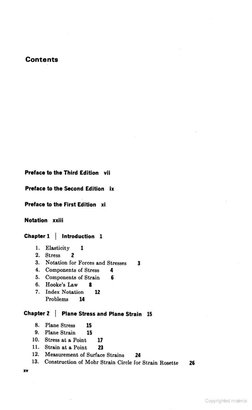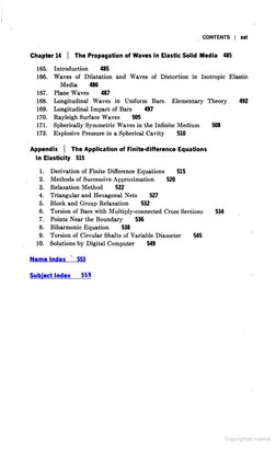Library of Congress Catalog Card Number 69-13617 ISBN-13: 978-0-07-070122-9 ISBN-10: 0-07-070122-9 Published by Tata McGraw Hill Education Private Limited, 7 West Patel Nagar, New Delhi 110 008, and printed at Sheel Print-N-Pack, Noida 201 305Contents Preface to the Third Edition vii Preface to the Second Edition ix Preface to the First Edition xi Notation xxiii Chapter1 | Introduction 1 Elasticity 1 Stress 2 Notation for Forces and Stresses 3 Components of Stress 4 Components of Strain 6 Hooke’s Law 8 Index Notation 12 Problems 14 Neopeye Chapter2 | Plane Stress and Plane Strain 15 8. Plane Stress 15 9. Plane Strain 15 10. Stress at a Point 7 IL. Strain ata Point 23 12, Measurement of Surface Strains a 13. 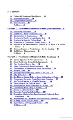Construction of Mohr Strain Circle for Strain Rosette 26xvi | CONTENTS 14. Differential Equations of Equilibrium 26 15. Boundary Conditions _28 16. Compatibility Equations 29 12_Stress Function __31 Problems _33 Chapter 3 I Two-dimensional Problems in Rectangular Coordinates 35 18. Solution by Polynomials 35 19._End Effects. Saint-Venant’s Principle 39 20. Determination of Displacements 40 21. Bending of a Cantilever Loaded at the End 41 22, Bending of a Beam by Uniform Load 46 23. Other Cases of Continuously Loaded Beams 50 24. Solution of the Two-dimensional Problem in the Form of a Fourier Series 53 25. Other Applications of Fourier Series. Gravity Loading 60 26. End Effects. Bigensolutions 61 Problems 63 Chapter 4 | Two-dimensional Problems in Polar Coordinates 65 27. General Equations in Polar Coordinates 65 28. Stress Distribution Symmetrical about an Axis 68 29. Pure Bending of Curved Bars 71 30. Strain Components in Polar Coordinates 75. 31. Displacements for Symmetrical Stress Distributions 77 -32. Rotating Disks 80 33. Bending of a Curved Bar by # Force at the End 83 34. Edge Dislocation _ 88 35. The Effect of Ci Hol 8 Distributions in:PL an 36. Concentrated Force at a Point of a Straight Boundary _97 37. Any Vertical Loading of a Straight Boundary _104 38. Force Acting on the End of a Wedge _109 39. Bending Couple Acting on the End of a Wedge —_112 40. Concentrated Force Acting ona Beam 113 s aS Di 12 2K Point ofan Infinite’ P Ww 3 Gi xed Bohition af the:*Twndi ional P Pol Coordinates __132 44. Applications of the Generalized Solution in Polar Coordinates 136 45. A Wedge Loaded’along the Faces 39 46. Eigensolutions for Wedges and Notches 41 Problems __144CONTENTS | xvil Chapter 5 | Photoelastic and Moiré Experimental Methods 150 Experimental Methods and Verifications 150 Photoelastic Stress Measurement 150 Circular Polariscope 155 Examples of Photoelastic Stress Determination 157 Determination of the Principal Stresses 160 Three-dimensional Photoelasticity 162 The Moiré Method 164 Chapter 6 | Two-dimensional Problems in Curvilinear Coordinates 168 54. Functions of a Complex Variable 168 55. Analytic Functions and Laplace’s Equation 170 Problems = 171. 56. Stress Functions in Terms of Harmonic and Complex Functions 172 57. Displacement Corresponding to a Given Stress Function 175 58. Stress and Displacement in Terms of Complex Potentials 176 59. Resultant of Stress on a Curve. Boundary Conditions 179 60. Curvilinear Coordinates 181 61. Stress Components in Curvilinear Coordinates 185 Problems 187 62. Solutions in Elliptic Coordinates. Elliptic Hole in Uniformly Stressed Plate 187 63. Elliptic Hole in a Plate under Simple Tension 191 64. Hyperbolic Boundaries. Notches 194 65. Bipolar Coordinates 196 66. Solutions in Bipolar Coordinates 198 Other Curvilinear Coordinates 202 Assignable Shapes 203 67. Determination of the Complex Potentials from Given Boundary Conditions. Methods of Muskhelishvili 203 68. Formulas for the Complex Potentials 206 69. Properties of Stress and Deformation Corresponding to Complex Poten- tials Analytic in the Material Region. around,a Hole 207 70. Theorems on Boundary Integrals 209 | 71. A Mapping Function w(t) for the Elliptic Hole, The Second Boundary Integral 212xvill, | CONTENTS 72. 73. The Elliptic Hole. Formula for ¥(é) a3 The Elliptic Hole. Particular Problems 26 Problems ay Chapter 7 | Analysis of Stress and Strain in Three Dimensions 219 Introduction ag Principal Stresses 221 . Stress Ellipsoid and Stress-director Surface 22 Determination of the Principal Stresses Stress Invariants 224 Determination of the Maximum Shearing Stress 224 Homogeneous Deformation 226 Strain ata Point 228 Principal Axes of Strain 231 Rotation 232 Problems 234 Chapter8 | General Theorems 235 84. 85. 86. 87. 88. 89. 90. 91. 92, 93. 94. 95. B38 Differential Equations of Equilibrium 235 Conditions of Compatibility 237 Determination of Displacements 240 Equations of Equilibrium in Terms of Displacements 240 General Solution for the Displacements 242 ‘The Principal of Superposition 243 Strain Energy 244 -Strain Energy of an Edge Dislocation 249 Principle of Virtual Work 250 Castigliano’s Theorem 254 Applications of the Principle of Least Work—Rectangular Plates 258 Effective Width of Wide Beam Flanges 262 Problems 268 Uniqueness of Solution 269 The Reciprocal Theorem 271 Approximate Character of the Plane Stress Solutions 274 Problems 2 Chapter9 | Elementary Problems of Elasticity in Three Dimensions 278 99. 100. Uniform Stress 278 Stretching of a Prismatical Bar by Its Own Weight 279101. 102. 103. CONTENTS | xix Twist of Circular Shafts of Constant Cross Section 282 Pure Bending of Prismatical Bars 284 Pure Bending of Plates 288 Chapter 10 | Torsion’ 291 104, 105, 106. 107. 108. 109. 110. lll. 112. 113, 114, 115. 116. iit. 118. 119. Torsion of Straight Bars 291 Elliptic Cross Section 297 Other Elementary Solutions 299 Membrane Anslogy 303 Torsion of a Bar of Narrow Rectangular Cross Section 307 Torsion of Rectangular Bars 309 Additional Results 313 Solution of Torsional Problems by Energy Method 315 Torsion of Rolled Profile Sections 321 Experimental Analogies 324 Hydrodynamicsl Analogies 325 Torsion of Hollow Shafts 328 Torsion of Thin Tubes 332 Screw Dislocations 336 Torsion of a Bar in Which One Cross Section Remains Plane 338 Torsion of Circular Shafts of Variable Diameter 341 Problems 349 Chapter 11 | Bending of Bars 354 120. 121, 122. 123. 124, 125. 126. 127. 128. 129. 130. Bending of a Cantilever 354 Stress Function 356 Circular Cross Section 358 Elliptic Cross Section 359 Rectangular Cross Section 361 Additional Results 366 Nonsymmetrical Cross Sections 369 Shear Center 371 The Solution of Bending Problems by the Soap-film Method 374 Displacements 378 Further Investigations of Bending 378 Chapter 12 | Axisymmetric Stress and Deformation in a Solid of Revolution 380 131. 182. 133. General Equations 380 Solution by Polynomials 383 Bending of a Circular Plate 385xx |- CONTENTS: 134. 135. 136. 137. 138. 139. 140. 141. 142. 143. 144. 145. 146. 147. The Rotating Disk as a Three-dimensional Problem 388 Force at @ Point in an Infinite Solid 390 Spherical Container under Internal or External Uniform Pressure 392. Local Stresses around a Spherical Cavity 396 Force on Boundary of a Semi-infinite Body 398 Load Distributed over a Part of the Boundary of a Semi-infinite Solid 403 Pressure between Two Spherical Bodies in Contact 409 Pressure between Two Bodies in Contact. More General Case 414 Impact of Spheres 420 Symmetrical Deformation of a Circular Cylinder 422 The Circular Cylinder with a Band of Pressure 425 Boussinesq’s Solution in Two Harmonic Functions 428 ‘The Helical Spring under Tension (Screw Dislocation ina Ring) 429 Pure Bending of an Incomplete Ring 432 Chapter 13 | Thermal Stress 433 148. 149. 151. 152. 153. 154. 155. 156. 157. 159. 160. 161. 162. 163. 164. The Simplest Cases of Thermal Stress Distribution. Method of Strain Suppression 433 Problems 438 Longitudinal Temperature Variation in a Strip 439 The Thin Circular Disk: Temperature Symmetrical about Center 441. The Long Circular Cylinder 443 Problems 452 The Sphere 452 General Equations 456 Thermoelastic Reciprocal Theorem 459 Overall Thermoelastic Deformations. Arbitrary Temperature Distribution 460 Thermoelastic Displacement. Maisel’s Integral Solution 463 Problems 466 Initial Stress 466 Total Volume Change Associated with Initial Stress 468 Plane Strain and Plane Stress. Method of Strain Suppression 469 ‘Two-dimensional Problems with Steady Heat Flow 470 Thermal Plane Stress Due to Disturbance of Uniform Heat Flow by an Insulated Hole ATS Solutions of the General Equations. Thermoelastic Displacement Potential 476 The General Two-dimensional Problem for Circular Regions 481 The: General Two-dimensional Problem in Complex Potentials 482CONTENTS | xi Chapter 14 | The Propagation of Waves in Elastic Solid Media 485 165. 166. 167. 168. 169. 170. 171. 172. Introduction 485 Waves of Dilatation and Waves of Distortion in Isotropic Elastic Media 486 Plane Waves 487 Longitudinal Waves in Uniform Bars. Elementary Theory 492 Longitudinal Impact of Bars 497. Rayleigh Surface Waves 505 Spherically Symmetric Waves in the Infinite Medium 508 Explosive Pressure in a Spherical Cavity 510 Appendix | The Application of Finite-difference Equations in Elasticity 515 be ee ol Derivation of Finite Difference Equations 515 Methods of Successive Approximation 520 Relaxation Method 522 Triangular and Hexagonal Nets 527 Block and Group Relaxation 532 Torsion of Bars with Multiply-connected Cross Sections 534 Points Near the Boundary 536 Biharmonic Equation 538 Torsion of Circular Shafts of Variable Diameter 545 Solutions by Digital Computer 549 s, Subject Index 559a You have either reached a page that is unavailable for viewing or reached your viewing limit for this book.a You have either reached a page that is unavailable for viewing or reached your viewing limit for this book.a You have either reached a page that is unavailable for viewing or reached your viewing limit for this book.a You have either reached a page that is unavailable for viewing or reached your viewing limit for this book.a You have either reached a page that is unavailable for viewing or reached your viewing limit for this book.a You have either reached a page that is unavailable for viewing or reached your viewing limit for this book.a You have either reached a page that is unavailable for viewing or reached your viewing limit for this book.a You have either reached a page that is unavailable for viewing or reached your viewing limit for this book.a You have either reached a page that is unavailable for viewing or reached your viewing limit for this book.a You have either reached a page that is unavailable for viewing or reached your viewing limit for this book.a You have either reached a page that is unavailable for viewing or reached your viewing limit for this book.a You have either reached a page that is unavailable for viewing or reached your viewing limit for this book.a You have either reached a page that is unavailable for viewing or reached your viewing limit for this book.a You have either reached a page that is unavailable for viewing or reached your viewing limit for this book.a You have either reached a page that is unavailable for viewing or reached your viewing limit for this book.a You have either reached a page that is unavailable for viewing or reached your viewing limit for this book.a You have either reached a page that is unavailable for viewing or reached your viewing limit for this book.a You have either reached a page that is unavailable for viewing or reached your viewing limit for this book.a You have either reached a page that is unavailable for viewing or reached your viewing limit for this book.a You have either reached a page that is unavailable for viewing or reached your viewing limit for this book.a You have either reached a page that is unavailable for viewing or reached your viewing limit for this book.a You have either reached a page that is unavailable for viewing or reached your viewing limit for this book.a You have either reached a page that is unavailable for viewing or reached your viewing limit for this book.a You have either reached a page that is unavailable for viewing or reached your viewing limit for this book.a You have either reached a page that is unavailable for viewing or reached your viewing limit for this book.a You have either reached a page that is unavailable for viewing or reached your viewing limit for this book.a You have either reached a page that is unavailable for viewing or reached your viewing limit for this book.a You have either reached a page that is unavailable for viewing or reached your viewing limit for this book.a You have either reached a page that is unavailable for viewing or reached your viewing limit for this book.2% | THEORY OF ELASTICITY m4 N # ¥ Fig. 20 In many practical applications the weight of the body is usually the only body force. Then, taking the y axis downward and denoting by p the mass per unit volume of the body, Eqs. (18) become O60, ote a toy 9) 15 | Boundary Conditions ‘Equations (18) or (19) must be satisfied at all points throughout the vol- ume of the body. The stress components vary over the volume of the plate; and when we arrive at the boundary they must be such as to be in equilibrium with the external forces on the boundary of the plate, so that external forces may be regarded as a continuation of the internal stress distribution. These conditions of equilibrium at the boundary can be obtained from Eqg. (12). Taking the small triangular prism PBC (Fig. 12), so that the side BC coincides with the boundary of the plate, as shown in Fig. 20, and denoting by X and Y the components of the surface forces per unit area at this point of the boundary, we have X =|, + mry Y¥ = my, + ry in which] and m are the direction cosines of the normal N to the boundary. In the particular case of a rectangular plate, the coordinate axes are usually taken parallel to the sides of the plate and the boundary condi- tions (20) can be simplified. Taking, for instance, a side of the plate parallel to the x axis we have for this part of the boundary the normal N parallel to the y axis; hence! = 0 and m = +1. Equations (20) then become (20) X=tm Yate Here the positive sign should be taken if the normal N has the positive direction of the y axis and the negative sign for the opposite directionPLANE STRESS AND PLANE STRAIN | 29 of N. It is seen from this that at the boundary the stress components become equal to the components of the surface forces per unit area of the boundary. 16 | Compatibility Equations It is a fundamental problem of the theory of elasticity to determine the state of stress in a body submitted to the action of given forces. In a two-dimensional problem it is necessary to solve the differential equa- tions of equilibrium (18), and the solution must be such as to satisfy the boundary conditions (20). These equations, derived by application of the equations of statics and containing three stress components 5, oy, Tay» are not sufficient for the determination of these components. ‘The prob- lem is a statically indeterminate one, and in order to obtain the solution the elastic deformation of the body must also be considered. The mathematical formulation of the condition for compatibility of stress distribution with the existence of continuous functions u, v, w defining the deformation will be obtained from Eqs. (2). For two- dimensional problems we consider three strain components, namely, = fo au, a =o & ay Yeu = oy at (a) These three strain components are expressed by two functions u and v; hence, they cannot be taken arbitrarily, and there exists a certain rela- tion between the strain components that can easily be obtained from (a). Differentiating the first of the Eqs. (a) twice with respect to y, the second twice with respect to z, and the third once with respect to z and once with respect to y, we find Oe, , Oey O*yzy ay? * dz? ~ az ay @) This differential relation, called the condition of compatibility, must be satisfied by the strain components to secure the existence of functions u and v connected with the strain components by Eqs. (a). By using Hooke’s law, [Eqs. (3)], the condition (21) ean be transformed into a relation between the components of stress. In the case of plane stress distribution (Art. 8), Eqs. (3) reduce to 1 1 f= ( — wy) = Ew (22) 1 yaa gr = Oe, (23)30 | THEORY OF ELASTICITY Substituting in Eq. (21), we find Srey oz oy This equation can be written in a different form by using the equations of equilibrium. For the case when the weight of the body is the only body force, differentiating the first of Eqs. (19) with respect to z and the second with respect to y and adding them, we find ae — voy) + Se — voz) = 2(1 + ») (b) Substituting in Eq. (6), the compatibility equation in terms of stress components becomes (+ 4) (+0) =0 (24) Proceeding in the same manner with the general equations of equilib- rium (18), we find +H) oto) =-at (X42 (25) (+) (+) In the case of plane strain (Art. 9), we have o, = voz +04) and from Hooke’s law (Eqs. 3), we find = Bl = Wee — H+ Nad 1 (26) = Bl — ey — 1 + Dor) ta = 20+, (27) Substituting in Eq. (21) and using, as before, the equations of equilib- rium (19), we find that the compatibility equation (24) holds also for plane strain. For the general case of body forces we obtain from Eqs. (21) and (18) the compatibility equation in the following form: a a ‘aX , oY (S+Z)er+o--+ G+ es) The equations of equilibrium (18) or (19) together with the boundary conditions (20) and one of the above compatibility equations give us a system of equations that is usually sufficient for the complete determi-PLANE STRESS AND PLANE STRAIN | 31 nation of the stress distribution in a two-dimensional problem.’ The particular cases in which certain additional considerations are necessary will be discussed later (page 133). It is interesting to note that in the case of constant body forces the equations determining stress distribution do not contain the elastic constants of the material. Hence, the stress distribution is the same for all isotropic materials, provided the equations are sufficient for the complete determination of the stresses. The con- clusion is of practical importance: we shall see later that in the case of transparent materials, such as glass or xylonite, it is possible to deter- mine stresses by an optical method using polarized light (page 150). From the above discussion it is evident that experimental results obtained with o transparent material in most cases can be applied immediately to any other material, such as steel. It should also be noted that in the case of constant body forces the compatibility equation (24) holds both for the case of plane stress and for the case of plane strain. The stress distribution is hence the same in these two cases, provided the shape of the boundary and the external forces are the same.” 17 | Stress Function It has been shown that a solution of two-dimensional problems reduces to the integration of the differential equations of equilibrium together with the compatibility equation and the boundary conditions. If we begin with the case when the weight of the body is the only body force, the equations to be satisfied are [see Eqs. (19) and (24)] dor | Oey at ty do, or, @ 0 Ory oy 7 oe +9 =0 ae oat oat aa) (z+ 0) =0 ) To these equations the boundary conditions (20) should be added. The usual method of solving these equations is by introducing a new function, 1In plane stress there are compatibility conditions other than (21) that are in fact violated by our assumptions. It is shown in Art. 131 that in spite of this the method of the present chapter gives good approximations for thin plates. 2 This statement may require modification when the plate or cylinder has holes, for then the problem can be correctly solved only by considering the displacements as well as the stresses. See Art. 43.32 | THEORY OF ELASTICITY called the stress function.! As is easily checked, Eqs. (a) are satisfied by taking any function ¢ of z and y and putting the following expressions for the stress components: a 9 _ _ 3% a= Oy m= gr Ut = — gy (29) In this manner we can get a variety of solutions of the equations of equi- librium (a). The true solution of the problem is that which satisfies also the compatibility equation (b). Substituting expressions (29) for the stress components into Eq. (b), we find that the stress function ¢ must. satisfy the equation oy byt Thus, the solution of a two-dimensional problem, when the weight of the body is the only, body force, reduces to finding a solution of Eq. (30) that satisfies the boundary conditions (20) of the problem. In the following chapters, this method of solution will be applied to several examples of practical interest. tg ote bat + 258 oy? + 0 (30) Let us now consider a more general case of body forces and assume that these forces have a potential. Then the components X and Y in Eqs. (18) are given by the equations © in which V is the potential function, Equations (18) become Zev +% =o Fa-n+%=0 Th +e equations are of the same form as Eqs. (a) and can be satisfied by taking ov = 38 «ov ~ Ss ra - SE @1) in whicl. 6 is the stress function. Substituting expressions (31) in the compatibility equation (25) for plane stress distribution, we find ge + 98-09 (SF +24) 82) dat ay + ay’ An analogous equation can be obtained for the case of plane strain. a gat? 1 This function was introduced in the solution of two-dimensional problems by G.B. Airy, Brit. Assoc. Advan. Sci. Repl., 1862, and is sometimes called the Airy stress function.PLANE STRESS AND PLANE STRAIN | 33 ‘When the body force is simply the weight, the potential V is —pgy. In this case the right-hand side of Eq. (32) reduces to zero. By taking the olution ¢ = Oof (32), or of (30), we find the stress distribution from (31), or (29), we- ey oy = ny ty = 0 @ asa possible state of stress due to gravity. ‘This is a state of hydrostatic pressure pgy in two dimensions, with zero stress at y = 0. It can exiat in a plate or cylinder of any shape provided the corresponding boundary forces are applied. Considering a bound- ary element as in Fig. 12, Eqs. (13) show that there must be normal pressure egy on the boundary, and sero shearetress. If the plate or cylinder is to be supported in some other manner we have to superpose a boundary normal tension egy and the new sup- porting forces. ‘The two together will be in equilibrium, and the determination of their effects ia a problem of boundary forces only, without body forces. PROBLEMS 1. Show that Ege. (12) remain velid when the element of Fig. 12 has acceleration. 2. Find grephically the principal strains and their directions from rosette measure- ments He =ZXW cary = 1.35 X10 easpay = 0.95 X 10-8 in, per in. where a = B = 45°. 3. Show that the line elements at the point 2, y that have the maximum and minimum rotation are those in the two perpendicular directions @ determined by av/ay — du/ax d0/ax + ou/ay 4. The stresses in a rotating disk (of unit thickness) can be regarded as due to cen- trifugal force as body force in a stationary disk. Show that this body force is derivable from the potential V = —3pu*(z' + y*), where p is the density and w the angular velocity of rotation (about the origin). 5. A disk with its axis horizontal has the gravity stress represented by Eqs. (d) of Art. 16. Make a sketch showing the boundary forces that support its weight. Show by another sketch the auxiliary problem of boundary forces that must be solved when the weight is entirely supported by the reaction of a horizontal surface on which the disk stands. 6. Accylinder with its axis horizontal has the gravity stress represented by Eqs. (d) of Art. 16. Its ends are confined between smooth fixed rigid planes that maintain the condition of plane strain. Sketch the forces acting on its surface, including the ends. 7. Using the strees-strain relations, and Eqs. (a) of Art. 15 in the equations of equi- librium (18), show that in the absence of body forces the displacements in problems of plane stress must satisfy au au l+»a /au ov eta rtia (+5) - and « companion equation. . tan 26 1 This problem, and the general case of a potential V such that the righthand side of Eq. (32) vanishes, have been discussed by M. Biot, J. Appl. Mech., 1935, p. A-41.34 | THEORY OF ELASTICITY 8. The figure represents a “tooth” on a plate in a state of plane stress in the plane of the paper. The faces of the tooth (the two straight lines) are free from force. On the supposition that the stress componenta are all finite and continuous throughout, the region, prove that there is no stress at all at the apex of the tooth.chapter 3 Two-dimensional Problems in Rectangular Coordinates 18 | Solution by Polynomials It has been shown that the solution of two-dimensional problems, when. body forces are absent or are constant, is reduced to the integration of the differential equation arg axt having regard to boundary conditions (20). In the case of long rec- tangular strips, solutions of Eq. (a) in the form of polynomials are of interest. By taking polynomials of various degrees, and suitably adjust- ing their coefficients, a number of practically important problems ean be solved.! Beginning with a polynomial of the second degree ag az* ay? +28 @9 (a) +? ay or = Fat + bay + oy ® which evidently satisfies Eq. (a), we find from Eqs. (29), putting pg = 0, a4: at a = Sp te oy = SB mo ta = — SE hs All three stress components are constant throughout the body, ie, the stress function (b) represents a combination of uniform tensions or com- pressions’ in two perpendicular directions and a uniform shear. The 1 A. Mesnager, Compt. Rend., vol. 132, p. 1475, 1901. See also A. Timpe, Z. Math. Physik, vol. 52, p. 348, 1905. + The arrows in Fig. 21 are all drawn in the standard sense, as defined in Art. 3. The numbers az, —bs, cs attached to them may be positive or negative. ‘Thu postibilities can be cor : however, the arrows show directly the intended directions of the applied forces. s36 | THEORY OF ELASTICITY ¥ Fig. 22 forces on the boundaries must equal the stresses at these points as dis- cussed on page 28; in the case of a rectangular plate with sides parallel to the coordinate axes, these forces are shown in Fig. 21. Let us consider now a stress function in the form of a polynomial of the third degree: t= sGyett Be + av + ath (©) This also satisfies Eq. (a). Using Eqs. (29) and putting pg = 0, we find on = SB = ose + dy oy = St aye + bay Ty = ze = —bar — cy For a rectangular plate, taken as in Fig. 22, assuming all coefficients except ds equal to zero, we obtain pure bending. If only coefficient a, is different from zero, we obtain pure bending by normal stresses applied to the sides y = tc of the plate. If coefficient bs or cs is taken different from zero, we obtain not only normal but also shearing stresses acting on the sides of the plate. Figure 23 represents, for instance, the case inTWO-DIMENSIONAL PROBLEMS IN RECTANGULAR COORDINATES | 37 which all coefficients except b; in function (c) are equal to zero. Along the sides y = tc we have uniformly distributed tensile and compressive stresses, respectively, and shearing stresses proportional to x. On the sidez = | we have only the constant shearing stress —bs/, and there are no stresses acting on the side z = 0. An analogous stress distribution is obtained if coefficient ¢: is taken different from zero. In taking the stress function in the form of polynomials of the second and third degrees we are completely free in choosing the magnitudes of the coefficients, since Eq. (a) is satisfied whatever values they may have. In the case of polynomials of higher degrees Eq. (a) is satisfied only if cer- tain relations between the coefficients are satisfied. Taking, for instance, the stress function in the form of a polynomial of the fourth degree, = Ot gy be oe te ee HTH tg tt tsqyw tae | and substituting it into Eq. (a), we find that the equation is satisfied only if 4 = —(2ca + a4) The stress components in this case are 2, a= 4 = can? + dary — (2c4 + ay? 2 y= ee = ag? + dary + cy? a 6, d, Rig ene — fat — 2eay — Fut Coefficients a, . . . , da in these expressions are arbitrary, and by suita- bly adjusting them we obtain various conditions of loading of a rectangu- lar plate. For instance, taking all coefficients except d, equal to zero, we find ea day 4 =0 ma Sy © e~dle { dl eo ' See “ a4 le y38 | THEORY OF ELASTICITY Assuming d, positive, the forces acting on the rectangular plate shown in Fig. 24 and producing the stresses (¢) are as given. On the longitudinal sides, y = +c are uniformly distributed shearing forces; on the ends, shearing forces are distributed according to a parabolic law. The shear- ing forces acting on the boundary of the plate reduce to the couple’ dct ldic? a> 2dl=5 2 act Mara 3 3-9 3 This couple balances the couple produced by the normal forces along the side z = 1 of the plate. Let us consider a stress function in the form of a polynomial of the fifth degree. _ a bs cs ds es Ss owe tae tse tag tig ta Substituting in Eq. (a) we find that this equation is satisfied if es = —(2cs + 3as) Ss = —34(bs + 2ds) The corresponding stress components are: ce 1 “Pars Bot + desty — (2es + Bas)ry* — 3 (Ds + 2ds)y* oy = Sb = ays + bey + cary? + yt a 1 ta = a = = gber? — coxty — deny? + 5 (2c5 + 3as)y? Again coefficients as, . .. , ds are arbitrary, and in adjusting them we obtain solutions for various loading conditions of a plate. Taking, for instance, all coefficients, except ds, equal to zero we find oz = ds(x’y — P4y?) : oy = Yedsy* @) = —dsry? Ty The normal forces are uniformly distributed along the longitudinal sides of the plate (Fig. 25a). Along the side x = |, the normal forces consist of two parts, one following a linear law and the other following the law of a 1 The thickness of the plate is taken equal to unity.TWO-DIMENSIONAL PROBLEMS IN RECTANGULAR COORDINATES | 39 cubic parabola. The shearing forces are proportional to z on the longi- tudinal sides of the plate and follow a parabolic law along the side z = 1. The distribution of these stresses is shown in Fig. 25b. ‘Since Eq. (a) is a linear differential equation, a sum of several solutions of this equation is also a solution. We can superpose the elementary solutions considered in this article to arrive at new solutions of practical interest. Several examples of the application of this method of super- position will be considered. 19 | End Effects. Saint-Venant’s Principle In the previous article several solutions for rectangular plates were obtained from very simple forms of the stress function ¢. In each case the boundary forces must be distributed exactly as the solution itself requires. In the case of pure bending, for instance (Fig. 22), the load- ing on the ends must consist of normal traction (¢., at x = 0 or z = 1) proportional to y. If the couples on the ends are applied in any other manner, the solution given in Art. 18 is no longer correct. Another solu- tion must be found if the changed boundary conditions on the ends are to be exactly satisfied. Many such solutions have been obtained (some are referred to later) not only for rectangular regions but for prismatic, cylindrical, and tapered shapes. These show that a change in the distri- bution'of the load on an end, without change of the resultant, alters the stress significantly only near the end. In such cases then, simple solu- tions such as those of the present chapter can give sufficiently accurate results except near the ends. The change of distribution of the load is equivalent to the super- position of a system of forces statically equivalent to zero force and zero couple. The expectation that such a system, applied to a small part of the surface of the body, would give rise to localized stress and strain only, was enunciated by Saint-Venant! in 1855 and came to be +B, de Saint-Venant, “Mémoires des Savants Etrangers,” vol. 14, 1855.40 | THEORY OF ELASTICITY known as Saint-Venanl’s principle. It accords with common experience in a variety of circumstances not confined to small strains in elastic materials obeying Hooke’s law—for instance, the application of a small clamp to a length of thick rubber tube causes appreciable strain only in the immediate neighborhood of the clamp. For bodies extended in two or three dimensions, such as disks, spheres, or the semi-infinite solid, the stress or strain due to loading on a small part of the body may be expected to diminish with distance on account of “geometrical divergence,” whether or not the resultant is zero. It has been shown! that vanishing of the resultant is not an adequate criterion for the degree of localization. 20 | Determination of Displacements When the components of stress are found from the previous equations, the components of strain can be obtained by using Hooke’s law, Eqs. (3) and (6). Then the displacements u and v can be obtained from the equations oH i, of ae By ou, dv ay tag = (a) The integration of these equations in each’ particular case does not pre- sent any difficulty, and we shall have several examples of their appli- cation. It may be seen at once that the strain components (a) remain unchanged if we add to u and v the linear functions — bt (b) in which a, 6, and ¢ are constants. This means that the displacements are not entirely determined by the stresses and strains. A displacement. like that of a rigid body can be superposed on the displacements due to the internal strains. The constants a and c in Eqs. (b) represent a trans- latory motion of the body and the constant b is a small angle of rotation of the rigid body about the 2 axis. It has been shown (see page 31) that in the case of constant body forces the stress distribution is the same for plane stress distribution or plane strain. The displacements are different for these two problems, however, since in the case of plane stress distribution the components of strain, entering into Eqs. (a), are given by equations waatby a= 1 eRe) a= Re) = Gt 'R, von Mises, Bull. Am. Math. Soc., vol. 51, p. 555, 1945; E. Sternberg, Quart. Appl. Math., vol. 11, p. 393, 1054; E. Sternberg and W. T. Koiter, J. Appl. Mech., vol. 25, pp. 575-581, 1958.TWO-DIMENSIONAL PROBLEMS IN RECTANGULAR COORDINATES | 41 and in the case of plane strain the strain components are: Jlee — vey + od] = lll = ree — 2 + Heal a= c= flor — vos + o)) = BIG = vey — 9 + oad 2 ‘Yer = GTav It is easily verified that these equations can be obtained from the pre- ceding -set for plane stress by replacing F in the latter by E/(1 — v*), and » by »/(1 — v). These substitutions leave G, which is B/2(1 + »), unchanged. The integration of Eqs. (a) will be shown later in discussing particular problems. a | Bending of a Cantilever Loaded at the End Consider a cantilever having a narrow rectangular cross section of unit width bent by force P applied at the end (Fig. 26). The upper and lower edges are free from load, and shearing forces, having a resultant P, are distributed along the end x = 0. These conditions can be satisfied by a proper combination of pure shear with the stresses (e) of Art. 18 represented in Fig. 24. Superposing the pure shear rz = —bz on the stresses (e), we find o. = day a,=0 (a) Ty = —ba — de ys To have the longitudinal sides y = +c free from forces we must have (rey) yee = —b2 -4e =0 " 2. t * Fe 4 x Fig. 2642 | THEORY OF ELASTICITY from which 2b; a= a To satisfy the condition on the loaded end the sum of the shearing forces distributed over this end must be equal to P. Hence! -f ra dy = f° (4-2) ay = P lg =e from which a3? eae Substituting these values of d, and bz in Eqs. (a) we find P : en ee 3P y E(B Noting that 2gc? is the moment of inertia J of the cross section of the cantilever, we have => oy =0 (b) Tay = —he-” This coincides completely with the elementary solution as given in books on the strength of materials. It should be noted that this solution repre- sents an exact solution only if the shearing forces on the ends are dis- tributed according to the same parabolic law as the shearing stress r1y and the intensity of the normal forces at, the built-in end is proportional toy. If the forces at the ends are distributed in any other manner, the stress distribution (b) is not a correct solution for the ends of the canti- lever, but, by virtue of Saint-Venant’s principle, it can be considered satisfactory for cross sections at a considerable distance from the ends. Let us consider now the displacement corresponding to the stresses (6). Applying Hooke’s law we find © (a) ' The minus sign before the integral follows from the rule for the sign of shearing stresses. Stress rzy on the end z = 0 is positive if it is upward (see p. 4).TWO-DIMENSIONAL PROBLEMS IN RECTANGULAR COORDINATES | 43 The procedure for obtaining the components u and v of the displacement consists in integrating Eqs. (c) and (d). By integration of Eqs. (c) we find _ _ Paty _ Pay? ua Seto = P+ A@ in which f(y) and f,(z) are as yet unknown functions of y only and z only. Substituting these values of u and v in Eq. (d) we find Go 4 oe +O . - ae) ~ art BEL In this equation some terms are functions of z only, some are functions of y only, and one is independent of both z and y. Denoting these groups by F(z), Gy), K, we have ans) GW) = YY) 4, Py _ Py F@ = — dy + 20 ~ 3G at Pet K= — a6 and the equation may be written FP) + Gy) = Such an equation means that F(z) must be some constant d and G(y) some constant e. Otherwise F(x) and G(y) would vary with z and y, respectively, and by varying z alone, or y alone, he equality would be violated. Thus Pe? etd=— 28 © aie) _ ze dy) _ _ »Py? , Py? ood dr Tt? “ay ~~ er tae t? Punetions f(y) and fx(z) are then _ Py, Py fo) = — Pe PP ey tg fie) = EE + de th Substituting in the expressions for u and v we find _ Paty _ Py un — Sat gar tag tate r 9) 0 ee Pe ath ~ QET 6EI“4 | THEORY OF ELASTICITY The constants d, e, g, h may now be determined from Eq. (e) and from the three conditions of constraint that are necessary to prevent the beam from moving as a rigid body in the zy plane. Assume that the point A, the centroid of the end cross section, is fixed. Then u and v are zero for x = 1, y = 0, and we find from Eqs. (g) _ _ _ PB g=0 he= eET dl The deflection curve is obtained by substituting y = 0 into the second of Eqs. (g). Then a(l— z) (h) For determining the constant d in this equation, we must use the third condition of constraint, eliminating the possibility of rotation of the beam in the zy plane about the fixed point A. This constraint can be realized in various ways. Let us consider two cases: (1) When an element of the axis of the beam is fixed at theend A. Then the condition of constraint is (Secs =f. # (2) When a vertical element of the cross section at the point A is fixed. Then the condition of constraint is du _ ess -° 9 In the first case we obtain from Eq. (A) PE a= — oer and from Eq. (e) we find = PP _ Pe °= DRT ~ 2G Substituting all the constants in Eqs. (g), we find = — Pry _ ay Py? (PE _ Per “= — SBT + arg * (oer ~ 376) ¥ da m,; = Pay, Pat Plz, Pit °= “oer ° Gel eI BET The equation of the deflection curve is Px? Pl'x , PU Wve = Er — Ser + SET (n)‘TWO-DIMENSIONAL PROBLEMS IN RECTANGULAR COORDINATES | 45 ) which gives for the deflection at the loaded end (x = 0) the value Pl'/ 3EI. This coincides with the value usually derived in elementary books on the strength of materials. To illustrate the distortion of cross sections produced by shearing stresses, let us consider the displacement u at the fixed end (x = 2). For this end we have from Eqs. (m), _ _ Py, Py _ Pey Oe = — GET + GIG ~ BIG au) _ Py? , Py? Pet & 1 ~ ter + 5G ~ 3G @ au) _ _ Pct_ BP au)iza = 7 IG = ~ EG The shape of the cross section after distortion is as shown in Fig. 27a. Owing to the shearing stress r-y = —3P/4e at. the point A, an element, of the cross section at A rotates in the zy plane about the point A through an angle 3P/4cG in the clockwise direction. If a vertical element of the cross section is fixed at A (Fig. 27b), instead. of a horizontal element of the axis, we find from condition (J) and the first of Eqs. (9) _ Pe * ORI and from Eq. (e) we find4% | THEORY OF ELASTICITY Substituting in the second of Eqs. (g) we find _ Ps? Pitz , PR | Pe ens = Er ~ ae + 3a7 + 216! - i Comparing this with Eq. (n) it can be concluded that, owing to rotation of the end of the axis at A (Fig. 276), the deflections of the axis of the cantilever are increased by the quantity Pe ap ged -D=Egl-» This is an estimate! of the so-called effect of shearing force on the deflec- tion of the beam. In practice, at the built-in end we have conditions different from those shown in Fig. 27. The fixed section? is usually not free to distort and the distribution of forces at this end is different from that given by Eqs. (b). However, solution (b) is satisfactory for com- paratively long cantilevers at considerable distances from the terminals. 22 | Bending of a Beam by Uniform Load Let a beam of narrow rectangular cross section of unit width, supported at the ends, be bent by a uniformly distributed load of intensity g, as shown in Fig. 28. The conditions at the upper and lower edges of the beam are: Cevate = 90 (y)yete = 0 (Os) ee = — 9 (@) The conditions at the ends z = +/ are [irvty= Fa [i oedy=0 fi aydy=0 The last two of Eqs. (b) state that there is no longitudinal force and no bending couple applied at the ends of the beam. All the conditions (a) * Others are indicated in Prob. 3, p. 63, and in the text on p. 49. The effect of elasticity in the support itself is examined experimentally and analytically by W. J. O'Donnell, J. Appl. Mech., vol. 27, pp. 461-464, 1960. he tT ray € SSS ¢ a @ (6) ) Fig. 28TWO-DIMENSIONAL PROBLEMS IN RECTANGULAR COORDINATES | 47 and (b) can be satisfied by combining certain solutions in the form of polynomials as obtained in Art. 18. We begin with solution (g), illus- trated by Fig. 25. To remove the tensile stresses along the side y = ¢ and the shearing stresses along the sides y = +c, we superpose a simple compression cy = a2 from solution (6), Art. 18, and the stresses o, = bsy and 72, = —bsx in Fig. 23. In this manner we find a. = de(uty — 3gy*) oy = Yedey* + by + a2 ©) Tay = —Adsxy? — bax From the conditions (a) we find —dy? —bs = 0 Yds + be +a. = 0 —Madsct — bie + a2 = —g from which wat wd anes Bony beg, ba ge Substituting in Eqs. (c) and noting that 2c?/3 is equal to the moment of inertia Z of the rectangular cross-sectional area of unit width, we find vn B8o-Hs) = 8-H) 2 = (br - evs 5 3 Tay = Zh (8 — yz = — 4 (— yz It can easily be checked that these stress components satisfy not only conditions (a) on the longitudinal sides but also the first two conditions (6) at the ends. To make the couples at the ends of the beam vanish, we superpose on solution (d) a pure bending, o: = day, o, = Try = 0, shown in Fig. 22, and determine the constant d; from the condition at z= 41 [iowa = f° [-35(y- Gr) + eu] ven =0 from which